Simulated Example Datasets From Baudry et al. (2010)

Simulated datasets used in Baudry et al. (2010) to illustrate the proposed mixture components combining method for clustering.

Please see the cited article for a detailed presentation of these datasets. The data frame with name exN.M is presented in Section N.M in the paper.

Test1D (not in the article) has been simulated from a Gaussian mixture distribution in R.

ex4.1 and ex4.2 have been simulated from a Gaussian mixture distribution in R^2.

ex4.3 has been simulated from a mixture of a uniform distribution on a square and a spherical Gaussian distribution in R^2.

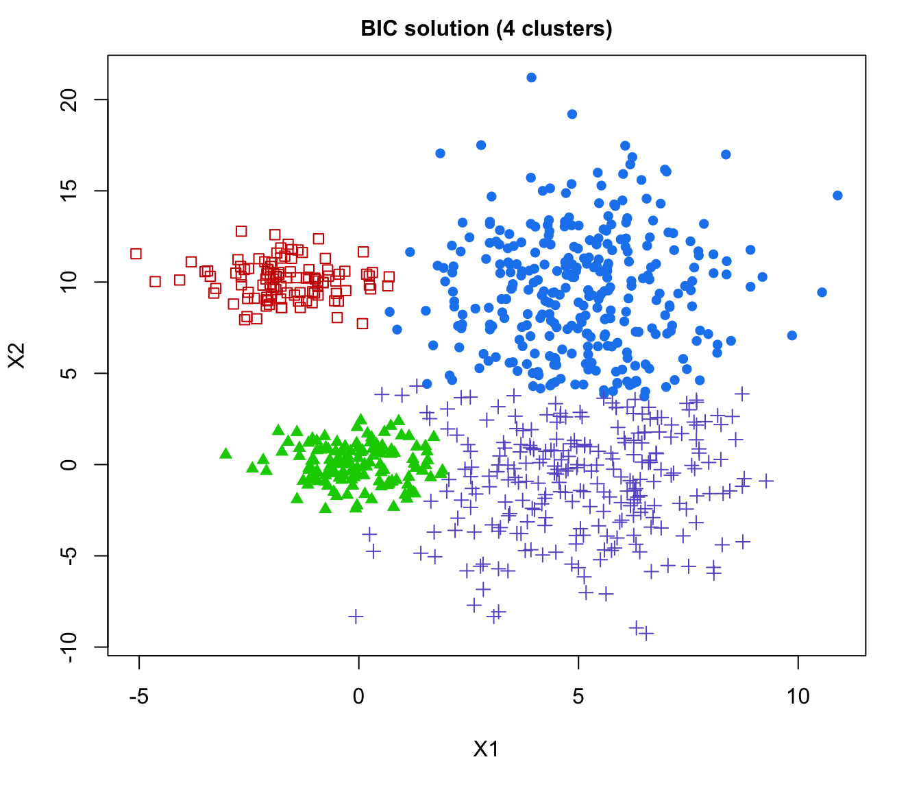
ex4.4.1 has been simulated from a Gaussian mixture model in R^2

ex4.4.2 has been simulated from a mixture of two uniform distributions in R^3.

Usage

data(Baudry_etal_2010_JCGS_examples)

Format

ex4.1 is a data frame with 600 observations on 2 real variables.

ex4.2 is a data frame with 600 observations on 2 real variables.

ex4.3 is a data frame with 200 observations on 2 real variables.

ex4.4.1 is a data frame with 800 observations on 2 real variables.

ex4.4.2 is a data frame with 300 observations on 3 real variables.

Test1D is a data frame with 200 observations on 1 real variable.

References

J.-P. Baudry, A. E. Raftery, G. Celeux, K. Lo and R. Gottardo (2010). Combining mixture components for clustering. Journal of Computational and Graphical Statistics, 19(2):332-353.

Examples

# \donttest{
data(Baudry_etal_2010_JCGS_examples)

output <- clustCombi(data = ex4.4.1)
output # is of class clustCombi
#> 'clustCombi' object:
#>  Mclust model: (VVI,4)
#>  Available object components: classification combiM combiz MclustOutput 
#>  Combining matrix (K+1 classes -> K classes): <object_name>$combiM[[K]]
#>  Classification for K classes: <object_name>$classification[[K]]

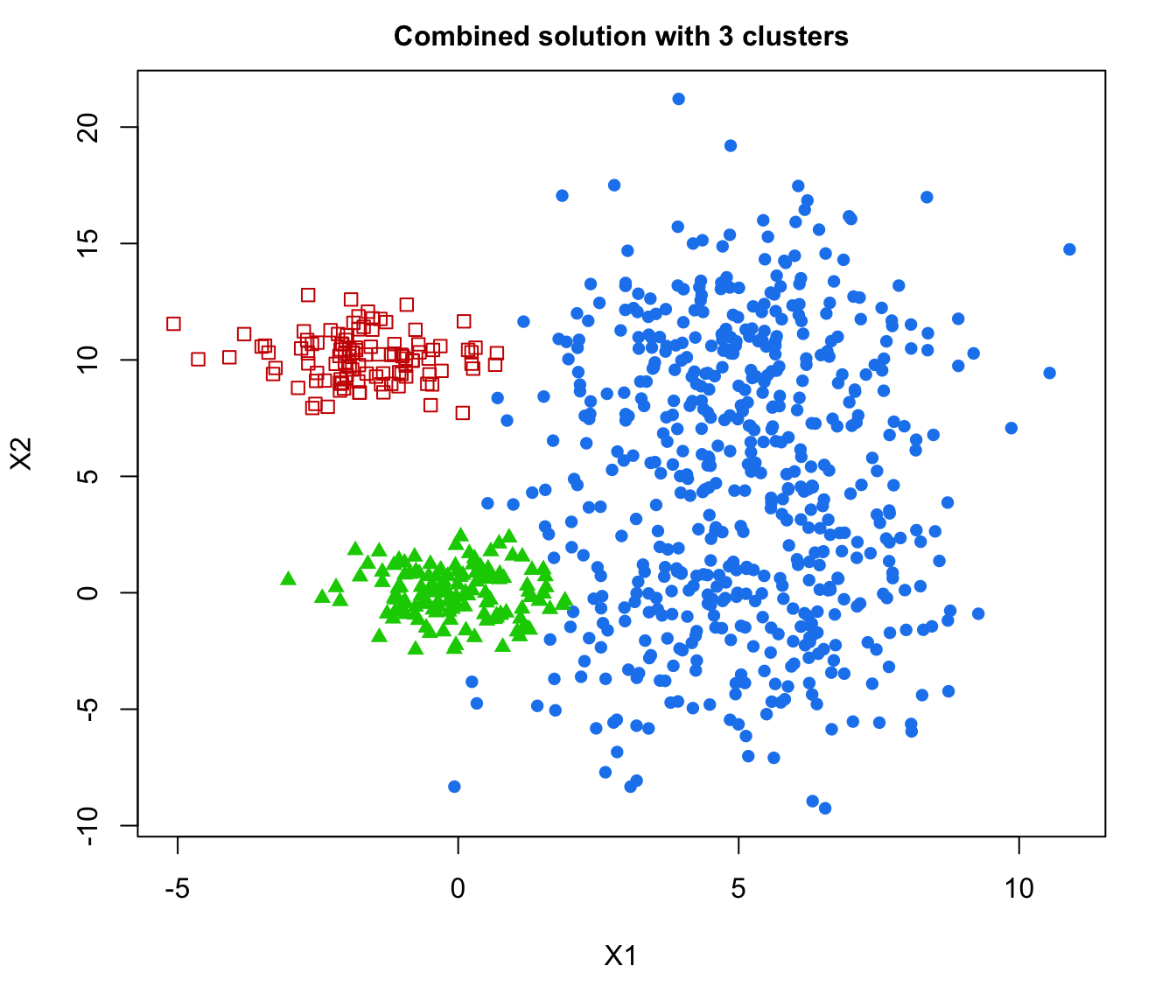
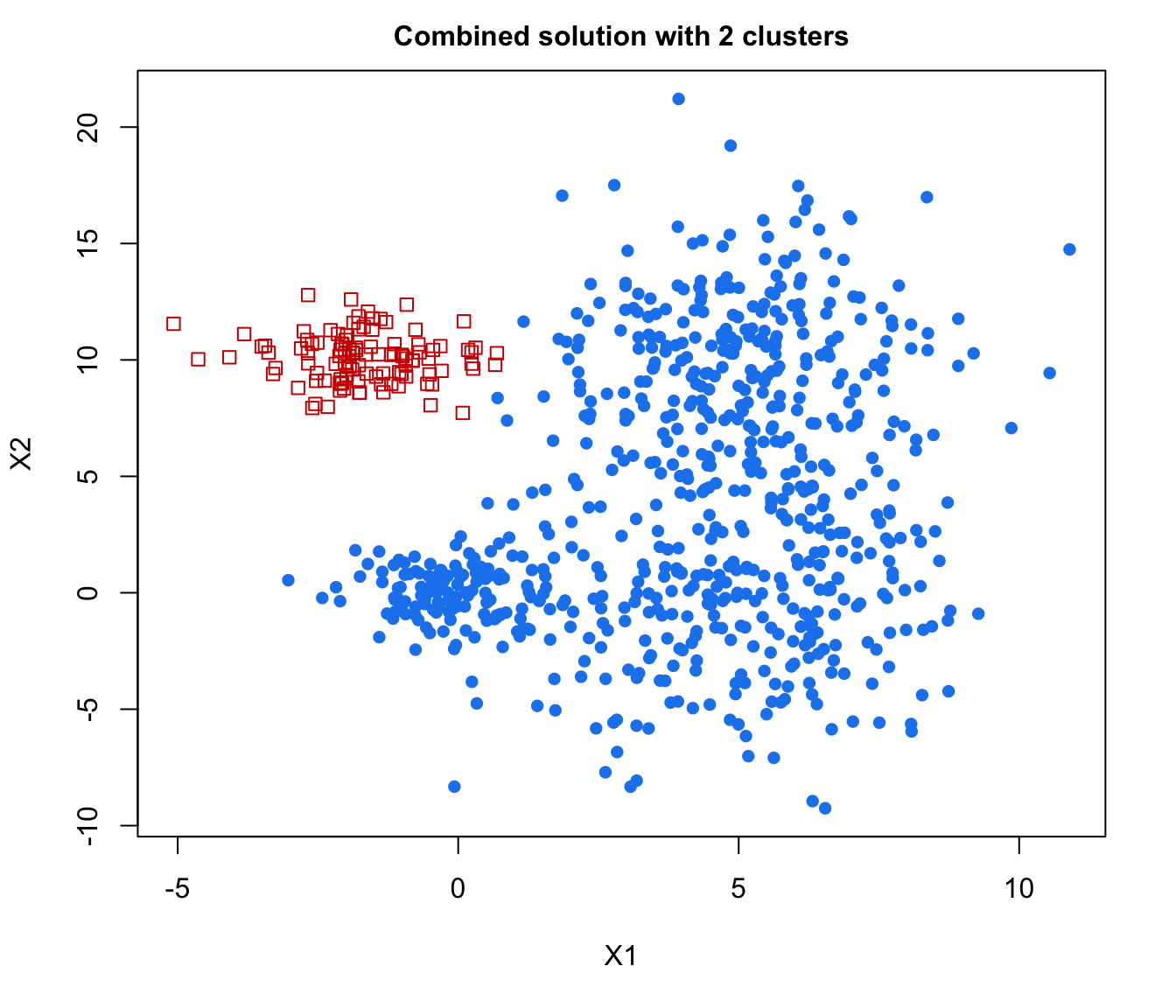
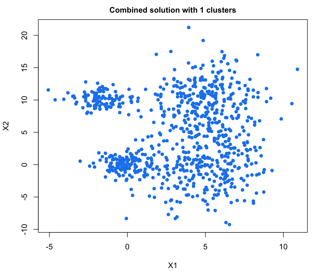
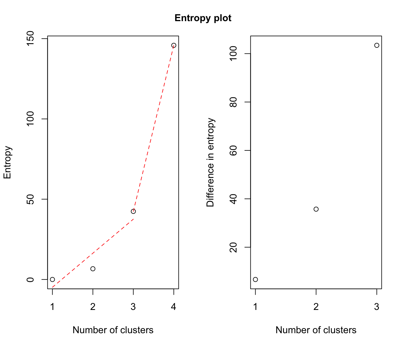
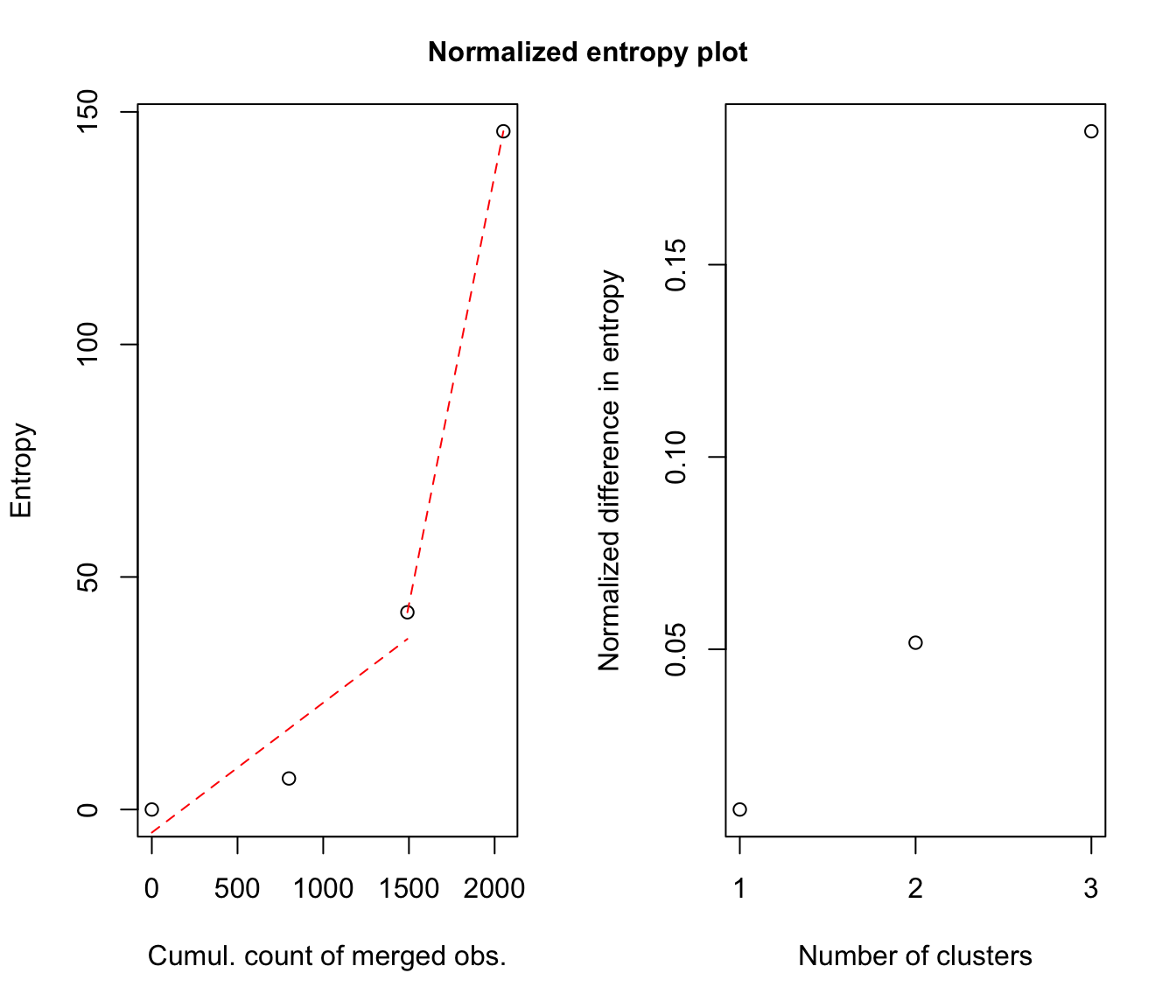
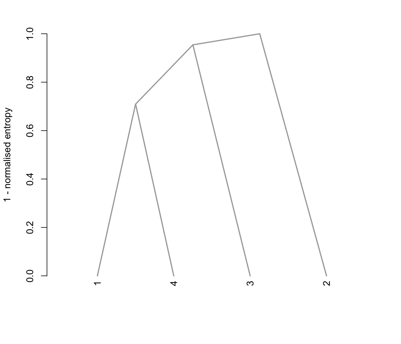
# plots the hierarchy of combined solutions, then some "entropy plots" which 
# may help one to select the number of classes
plot(output) 







# }