Cumulative distribution and quantiles of univariate model-based mixture density estimation for bounded data

Compute the cumulative density function (cdf) or quantiles of a one-dimensional density for bounded data estimated via transformation-based approach for Gaussian mixtures using densityMclustBounded.

Usage

cdfDensityBounded(object, data, ngrid = 100, ...)
quantileDensityBounded(object, p, ...)

Arguments

object: a densityMclustBounded model object.
data: a numeric vector of evaluation points.
ngrid: the number of points in a regular grid to be used as evaluation points if no data are provided.
p: a numeric vector of probabilities.
...: further arguments passed to or from other methods.

Details

The cdf is evaluated at points given by the optional argument data. If not provided, a regular grid of length ngrid for the evaluation points is used.

The quantiles are computed using bisection linear search algorithm.

Value

cdfDensityBounded returns a list of x and y values providing, respectively, the evaluation points and the estimated cdf.

quantileDensityBounded returns a vector of quantiles.

Author

Luca Scrucca

Examples

# \donttest{
# univariate case with lower bound
x <- rchisq(200, 3)
dens <- densityMclustBounded(x, lbound = 0)

xgrid <- seq(-2, max(x), length=1000)
cdf <- cdfDensityBounded(dens, xgrid)
str(cdf)
#> List of 2
#>  $ x: num [1:1000] -2 -1.98 -1.96 -1.95 -1.93 ...
#>  $ y: num [1:1000] 0 0 0 0 0 0 0 0 0 0 ...
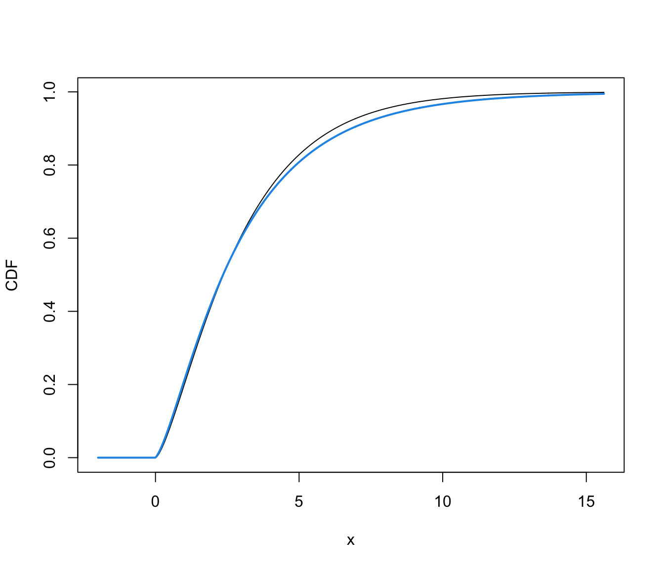
plot(xgrid, pchisq(xgrid, df = 3), type = "l", xlab = "x", ylab = "CDF")
lines(cdf, col = 4, lwd = 2)


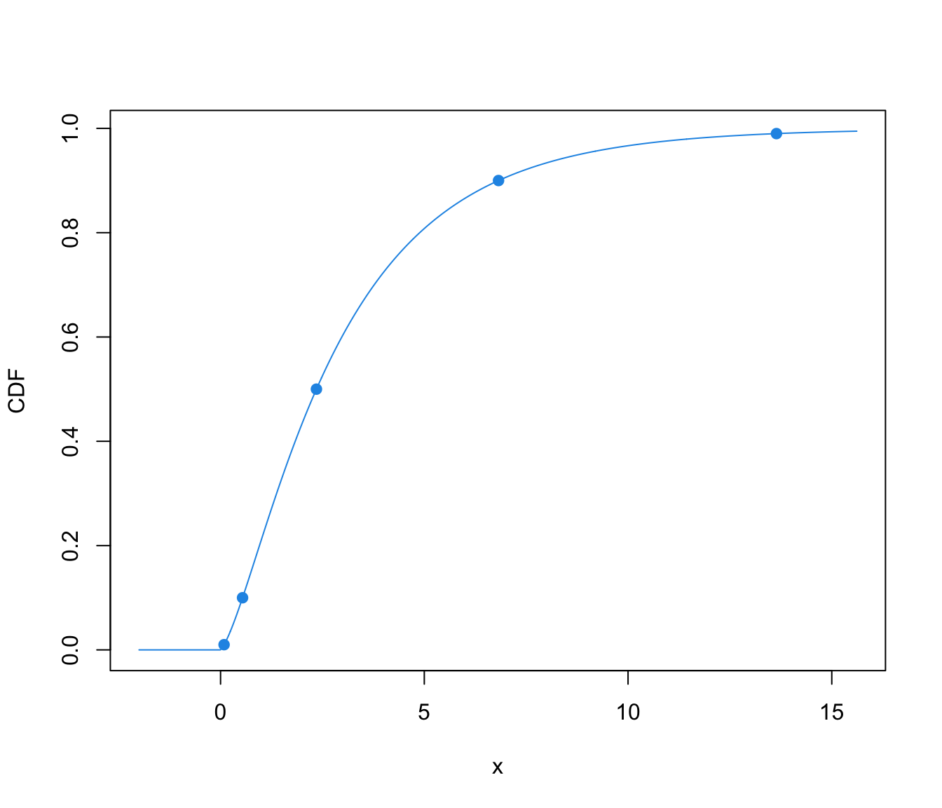
q <- quantileDensityBounded(dens, p = c(0.01, 0.1, 0.5, 0.9, 0.99))
cbind(quantile = q, cdf = cdfDensityBounded(dens, q)$y)
#>         quantile  cdf
#> [1,]  0.08635328 0.01
#> [2,]  0.53968005 0.10
#> [3,]  2.35284217 0.50
#> [4,]  6.82174271 0.90
#> [5,] 13.64201527 0.99
plot(cdf, type = "l", col = 4, xlab = "x", ylab = "CDF")
points(q, cdfDensityBounded(dens, q)$y, pch = 19, col = 4)


# univariate case with lower & upper bounds
x <- rbeta(200, 5, 1.5)
dens <- densityMclustBounded(x, lbound = 0, ubound = 1)

xgrid <- seq(-0.1, 1.1, length=1000)
cdf <- cdfDensityBounded(dens, xgrid)
str(cdf)
#> List of 2
#>  $ x: num [1:1000] -0.1 -0.0988 -0.0976 -0.0964 -0.0952 ...
#>  $ y: num [1:1000] 0 0 0 0 0 0 0 0 0 0 ...
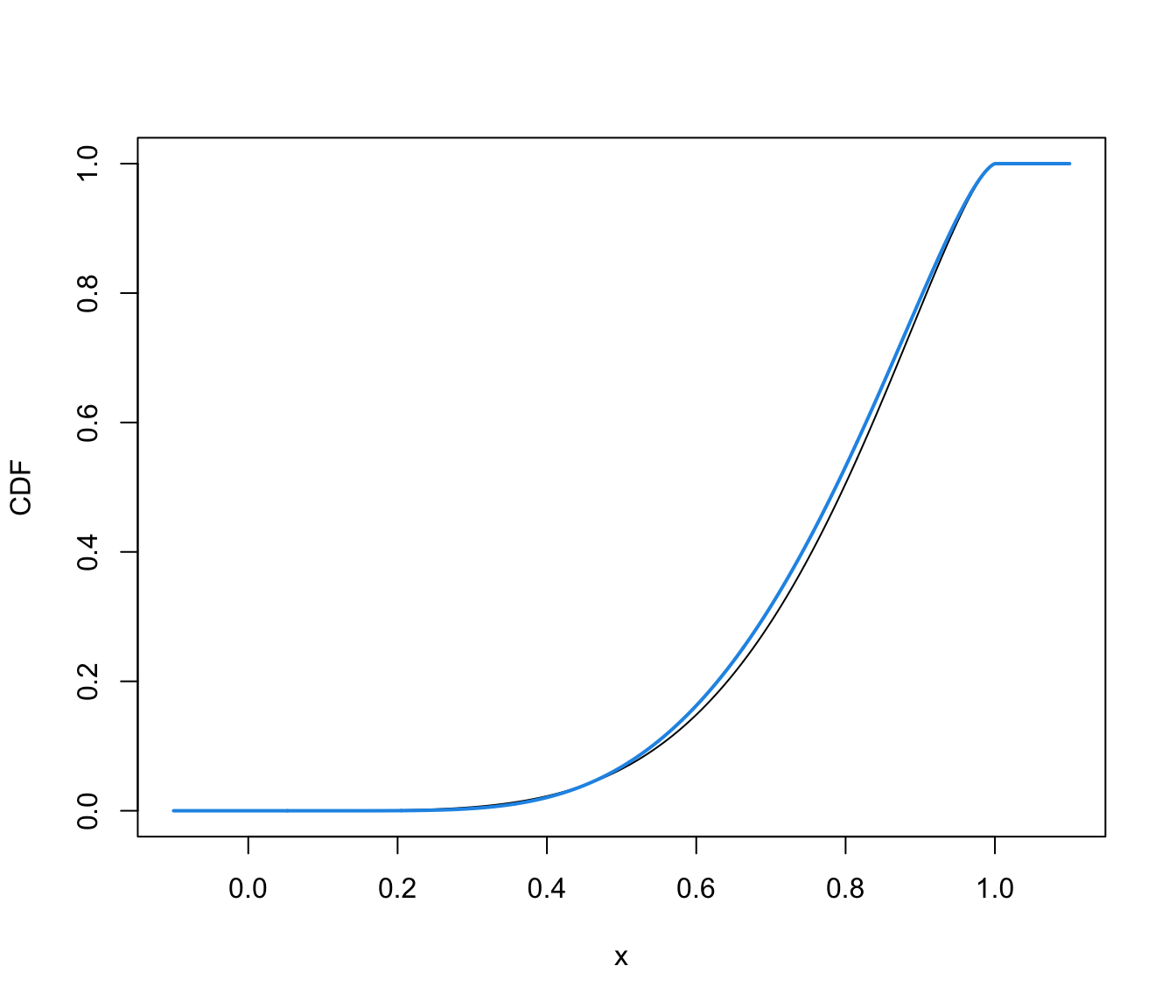
plot(xgrid, pbeta(xgrid, 5, 1.5), type = "l", xlab = "x", ylab = "CDF")
lines(cdf, col = 4, lwd = 2)


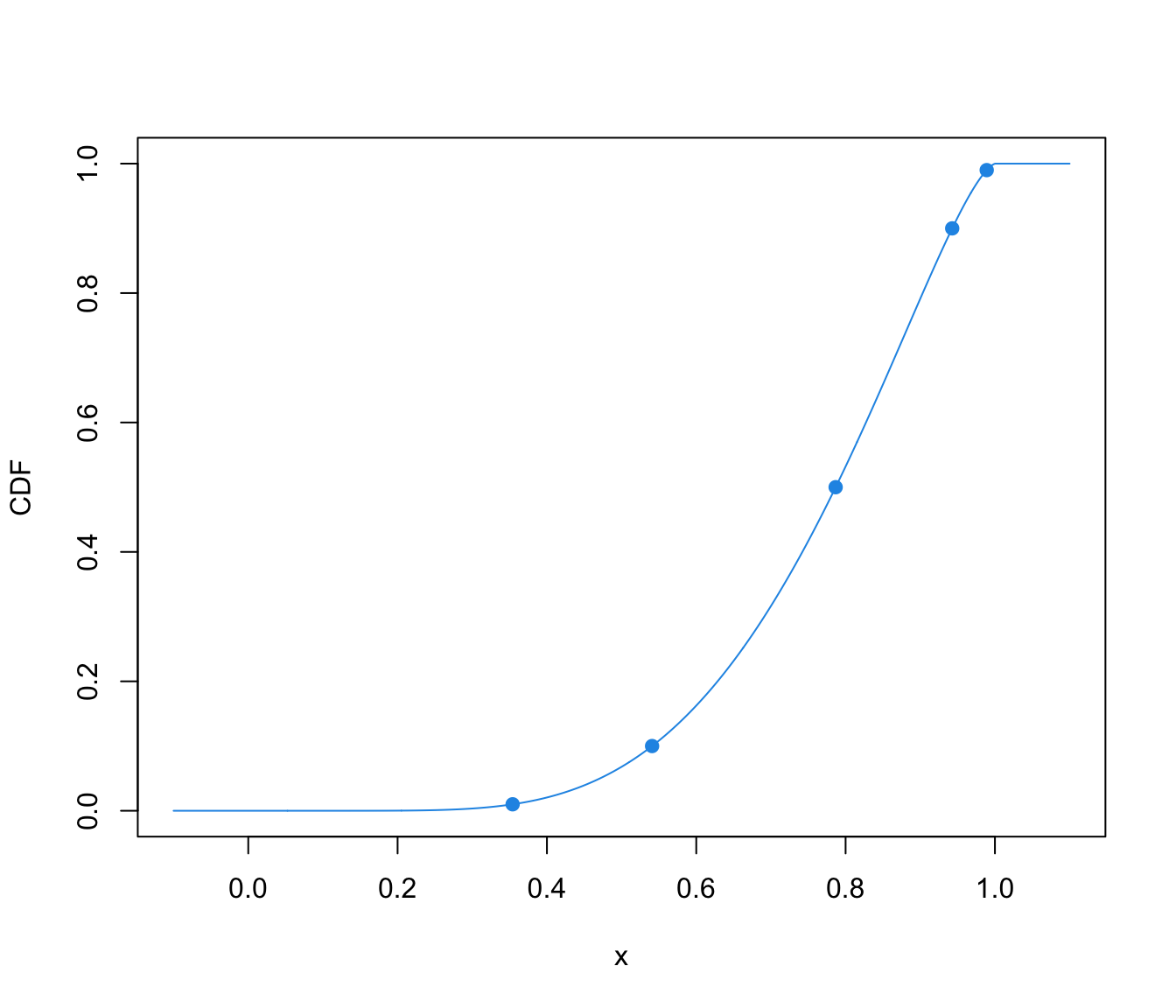
q <- quantileDensityBounded(dens, p = c(0.01, 0.1, 0.5, 0.9, 0.99))
cbind(quantile = q, cdf = cdfDensityBounded(dens, q)$y)
#>       quantile  cdf
#> [1,] 0.3540720 0.01
#> [2,] 0.5408286 0.10
#> [3,] 0.7866718 0.50
#> [4,] 0.9427872 0.90
#> [5,] 0.9889984 0.99
plot(cdf, type = "l", col = 4, xlab = "x", ylab = "CDF")
points(q, cdfDensityBounded(dens, q)$y, pch = 19, col = 4)

# }