Model-based mixture density estimation for bounded data

Density estimation for bounded data via transformation-based approach for Gaussian mixtures.

Usage

densityMclustBounded(data, 
                     G = NULL, modelNames = NULL,
                     lbound = NULL, 
                     ubound = NULL, 
                     lambda = c(-3, 3),
                     prior = NULL,
                     noise = NULL,
                     nstart = 25,
                     parallel = FALSE,
                     seed = NULL,
                     ...)

# S3 method for densityMclustBounded
print(x, digits = getOption("digits"), ...)

# S3 method for densityMclustBounded
summary(object, parameters = FALSE, classification = FALSE, ...)

Arguments

data

A numeric vector, matrix, or data frame of observations. If a matrix or data frame, rows correspond to observations and columns correspond to variables.

G

An integer vector specifying the numbers of mixture components. By default G=1:3.

modelNames

A vector of character strings indicating the Gaussian mixture models to be fitted on the transformed-data space. See mclustModelNames for a descripton of available models.

lbound

Numeric vector proving lower bounds for variables.

ubound

Numeric vector proving upper bounds for variables.

lambda

A numeric vector providing the range of searched values for the transformation parameter(s).

prior

A function specifying a prior for Bayesian regularization of Gaussian mixtures. See priorControl for details.

noise

A specification for the noise component. Currently, not available.

nstart

An integer value specifying the number of replications of k-means clustering to be used for initializing the EM algorithm. See kmeans.

parallel

An optional argument which allows to specify if the search over all possible models should be run sequentially (default) or in parallel.

For a single machine with multiple cores, possible values are:

a logical value specifying if parallel computing should be used (TRUE) or not (FALSE, default) for evaluating the fitness function;
a numerical value which gives the number of cores to employ. By default, this is obtained from the function detectCores;
a character string specifying the type of parallelisation to use. This depends on system OS: on Windows OS only "snow" type functionality is available, while on Unix/Linux/Mac OSX both "snow" and "multicore" (default) functionalities are available.

In all the cases described above, at the end of the search the cluster is automatically stopped by shutting down the workers.

If a cluster of multiple machines is available, evaluation of the fitness function can be executed in parallel using all, or a subset of, the cores available to the machines belonging to the cluster. However, this option requires more work from the user, who needs to set up and register a parallel back end. In this case the cluster must be explicitely stopped with stopCluster.

seed

An integer value containing the random number generator state. This argument can be used to replicate the result of k-means initialisation strategy. Note that if parallel computing is required, the doRNG package must be installed.

x, object

An object of class "densityMclustBounded".

digits

The number of significant digits to use for printing.

parameters

Logical; if TRUE, the parameters of mixture components are printed.

classification

Logical; if TRUE, the MAP classification/clustering of observations is printed.

...

Further arguments passed to or from other methods.

Value

Returns an object of class "densityMclustBounded".

Author

Luca Scrucca

References

Scrucca L. (2019) A transformation-based approach to Gaussian mixture density estimation for bounded data. Biometrical Journal, 61:4, 873–888. https://doi.org/10.1002/bimj.201800174

Examples

# \donttest{
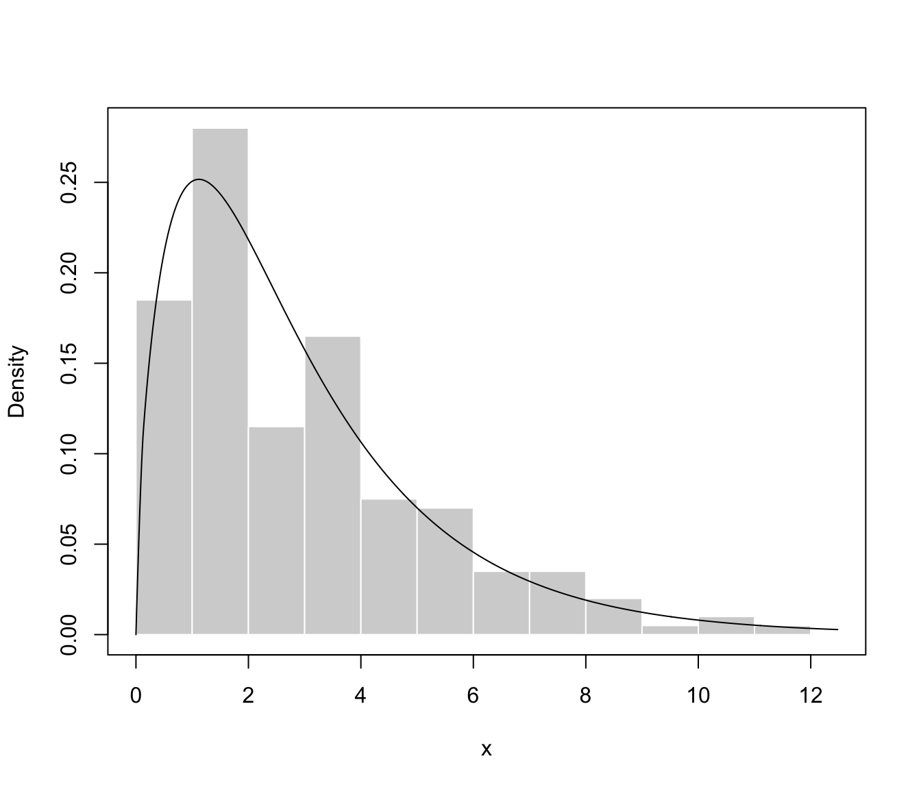
# univariate case with lower bound
x <- rchisq(200, 3)
xgrid <- seq(-2, max(x), length=1000)
f <- dchisq(xgrid, 3)  # true density
dens <- densityMclustBounded(x, lbound = 0)
summary(dens)
#> ── Density estimation for bounded data via GMMs ─────────── 
#>            
#> Boundaries:   x
#>       lower   0
#>       upper Inf
#> 
#> Model E (univariate, equal variance) model with 1 component
#> on the transformation scale:
#> 
#>  log-likelihood   n df       BIC       ICL
#>       -407.3154 200  3 -830.5257 -830.5257
#> 
#>                                     x
#> Range-power transformation: 0.2730149
summary(dens, parameters = TRUE)
#> ── Density estimation for bounded data via GMMs ─────────── 
#>            
#> Boundaries:   x
#>       lower   0
#>       upper Inf
#> 
#> Model E (univariate, equal variance) model with 1 component
#> on the transformation scale:
#> 
#>  log-likelihood   n df       BIC       ICL
#>       -407.3154 200  3 -830.5257 -830.5257
#> 
#>                                     x
#> Range-power transformation: 0.2730149
#> 
#> Mixing probabilities:
#> 1 
#> 1 
#> 
#> Means:
#>         1 
#> 0.9492891 
#> 
#> Variances:
#>        1 
#> 1.183863 
plot(dens, what = "BIC")

plot(dens, what = "density")
lines(xgrid, f, lty = 2)

plot(dens, what = "density", data = x, breaks = 15)


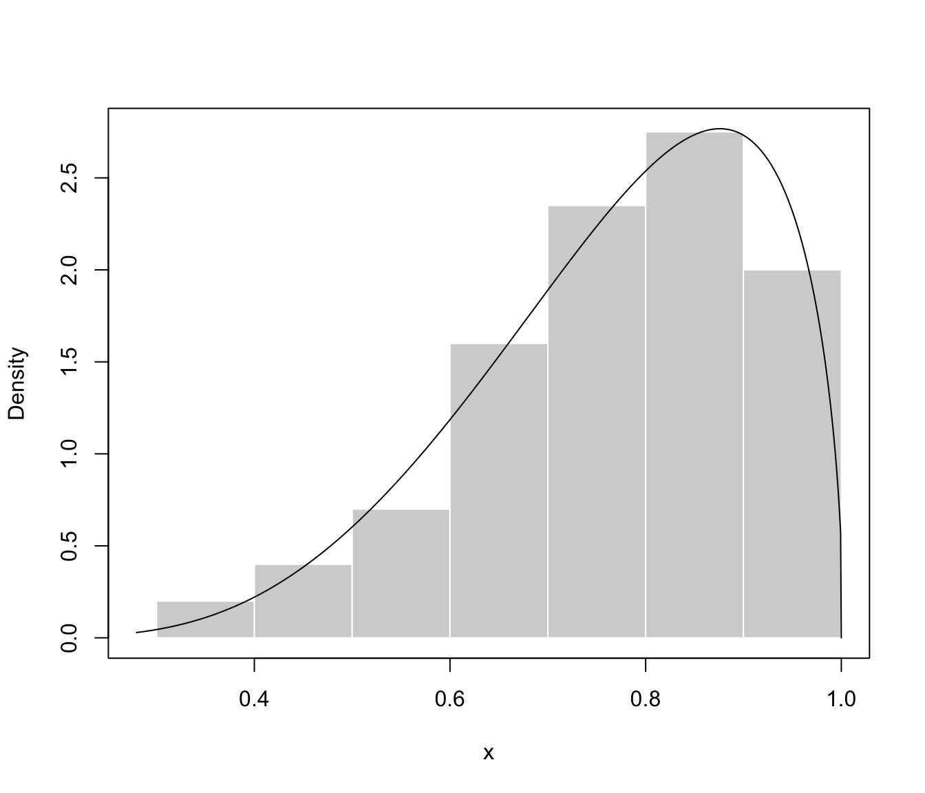
# univariate case with lower & upper bounds
x <- rbeta(200, 5, 1.5)
xgrid <- seq(-0.1, 1.1, length=1000)
f <- dbeta(xgrid, 5, 1.5)  # true density
dens <- densityMclustBounded(x, lbound = 0, ubound = 1)
summary(dens)
#> ── Density estimation for bounded data via GMMs ─────────── 
#>            
#> Boundaries: x
#>       lower 0
#>       upper 1
#> 
#> Model E (univariate, equal variance) model with 1 component
#> on the transformation scale:
#> 
#>  log-likelihood   n df      BIC      ICL
#>        121.6621 200  3 227.4293 227.4293
#> 
#>                                     x
#> Range-power transformation: -0.227797
plot(dens, what = "BIC")

plot(dens, what = "density")

plot(dens, what = "density", data = x, breaks = 9)


# bivariate case with lower bounds
x1 <- rchisq(200, 3)
x2 <- 0.5*x1 + sqrt(1-0.5^2)*rchisq(200, 5)
x <- cbind(x1, x2)
plot(x)

dens <- densityMclustBounded(x, lbound = c(0,0))
summary(dens, parameters = TRUE)
#> ── Density estimation for bounded data via GMMs ─────────── 
#>            
#> Boundaries:  x1  x2
#>       lower   0   0
#>       upper Inf Inf
#> 
#> Model EEE (ellipsoidal, equal volume, shape and orientation) model with 2 components
#> on the transformation scale:
#> 
#>  log-likelihood   n df       BIC       ICL
#>       -848.3453 200 10 -1749.674 -1777.231
#> 
#>                                    x1        x2
#> Range-power transformation: 0.2439339 0.3001117
#> 
#> Mixing probabilities:
#>         1         2 
#> 0.2186624 0.7813376 
#> 
#> Means:
#>            [,1]     [,2]
#> [1,] 0.06442665 1.080146
#> [2,] 2.78470340 1.815451
#> 
#> Variances:
#> [,,1]
#>           [,1]      [,2]
#> [1,] 0.9661706 0.5514568
#> [2,] 0.5514568 0.6529538
#> [,,2]
#>           [,1]      [,2]
#> [1,] 0.9661706 0.5514568
#> [2,] 0.5514568 0.6529538
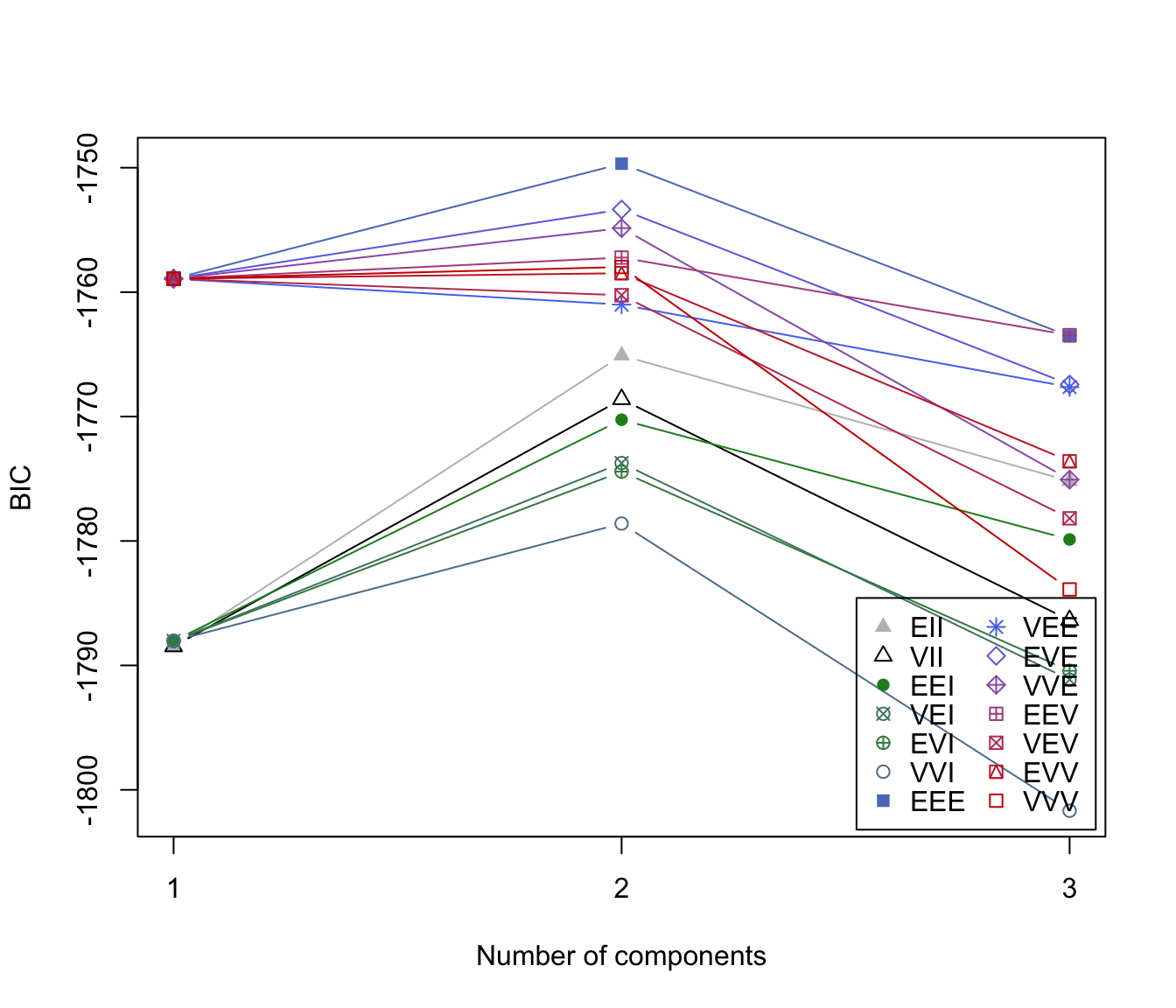
plot(dens, what = "BIC")

plot(dens, what = "density")

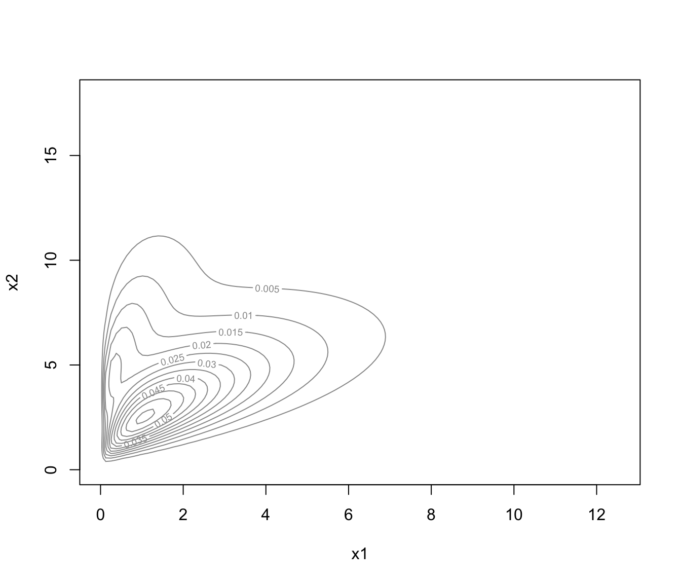plot(dens, what = "density", type = "hdr")

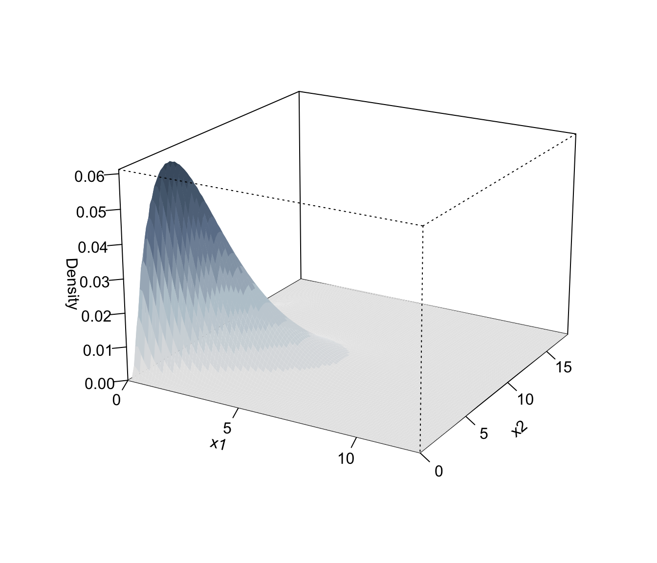
plot(dens, what = "density", type = "persp")

# }