Cumulative distribution and quantiles of univariate model-based mixture density estimation for bounded data

Compute the cumulative density function (cdf) or quantiles of a one-dimensional density for bounded data estimated via the transformation-based approach for Gaussian mixtures in densityMclustBounded().

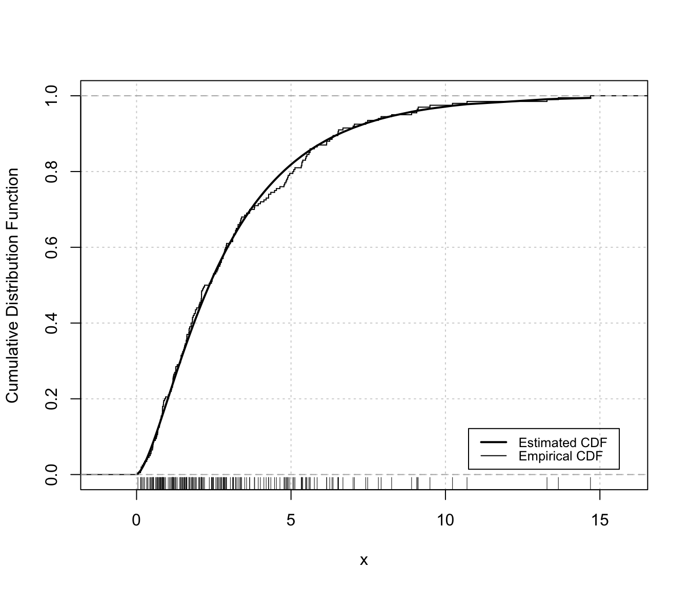
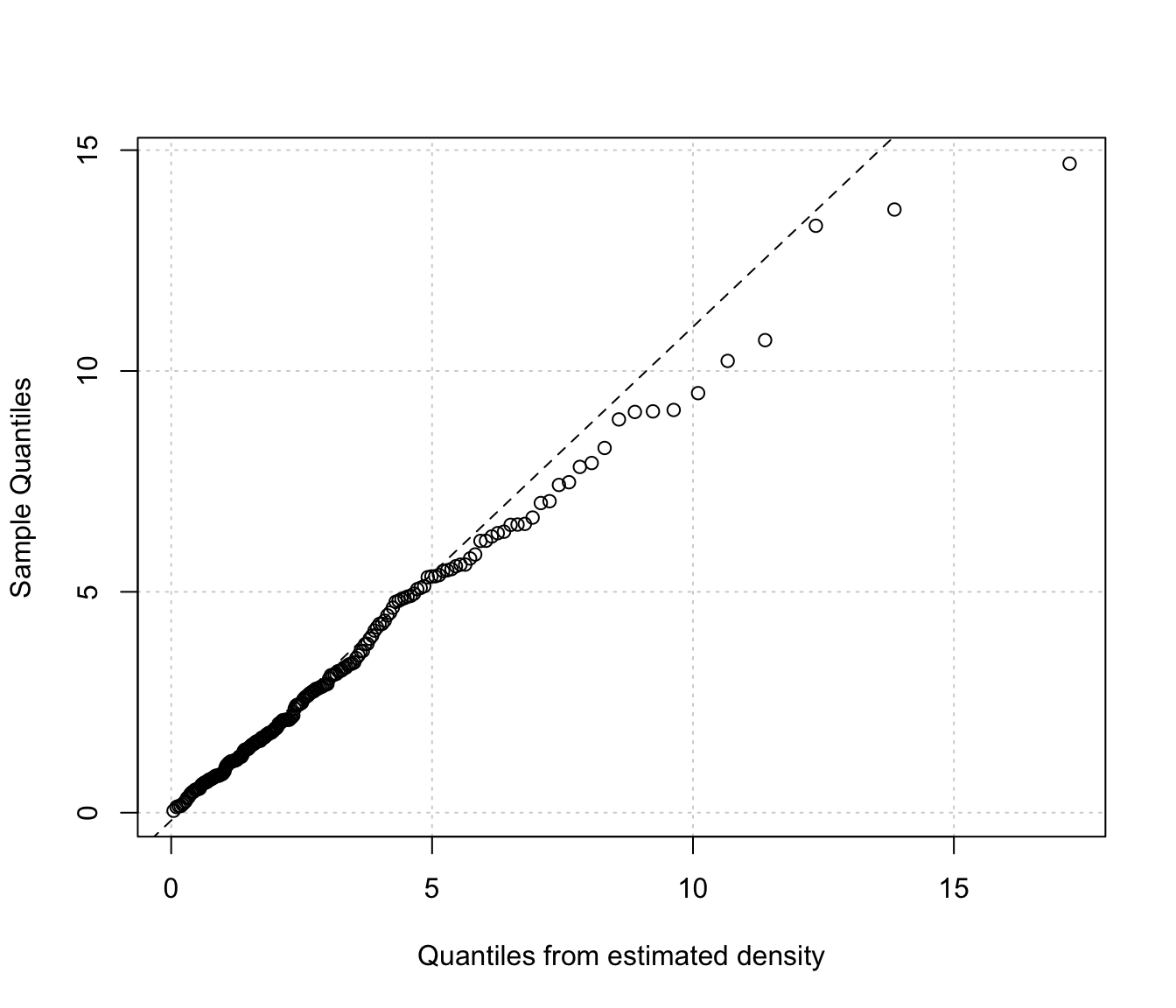
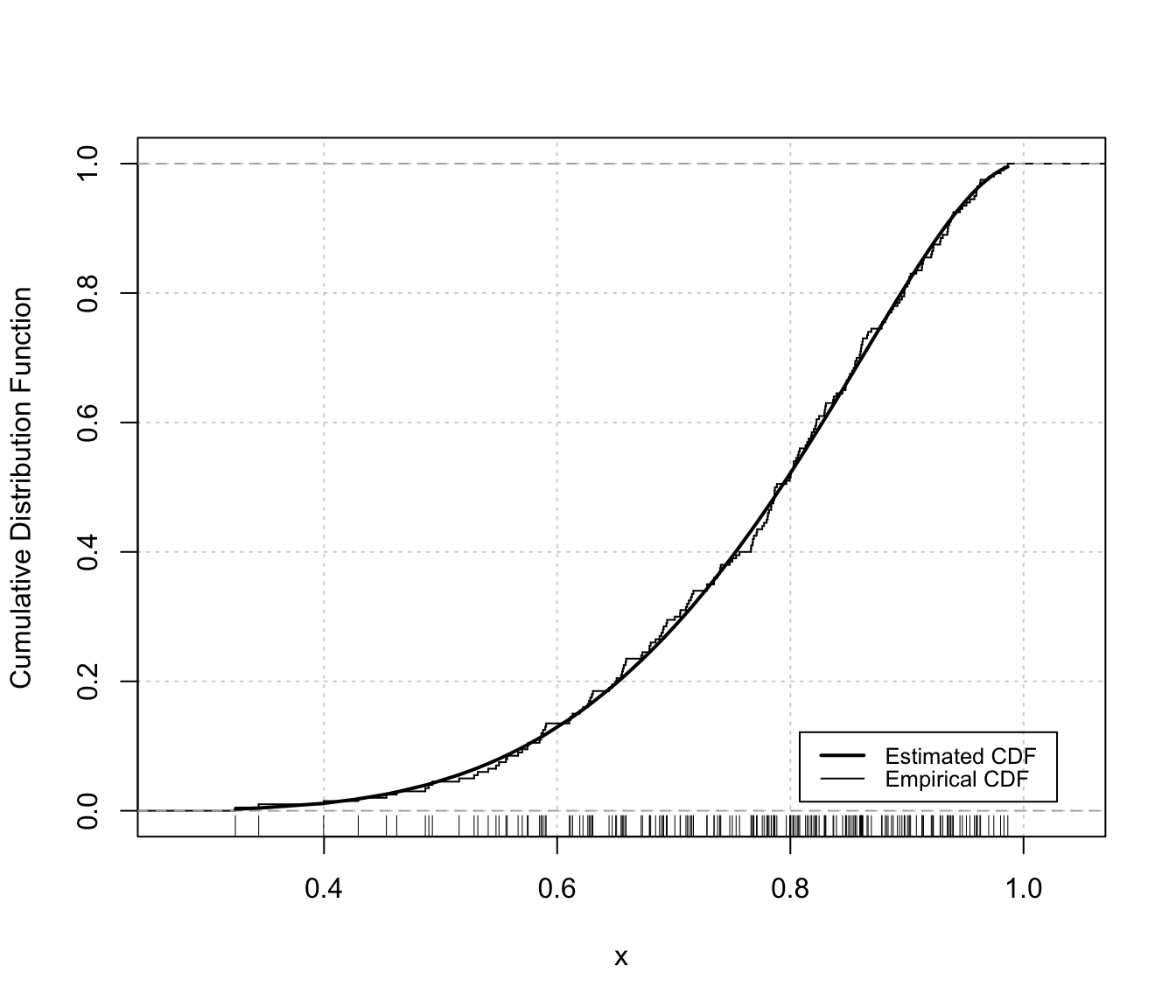
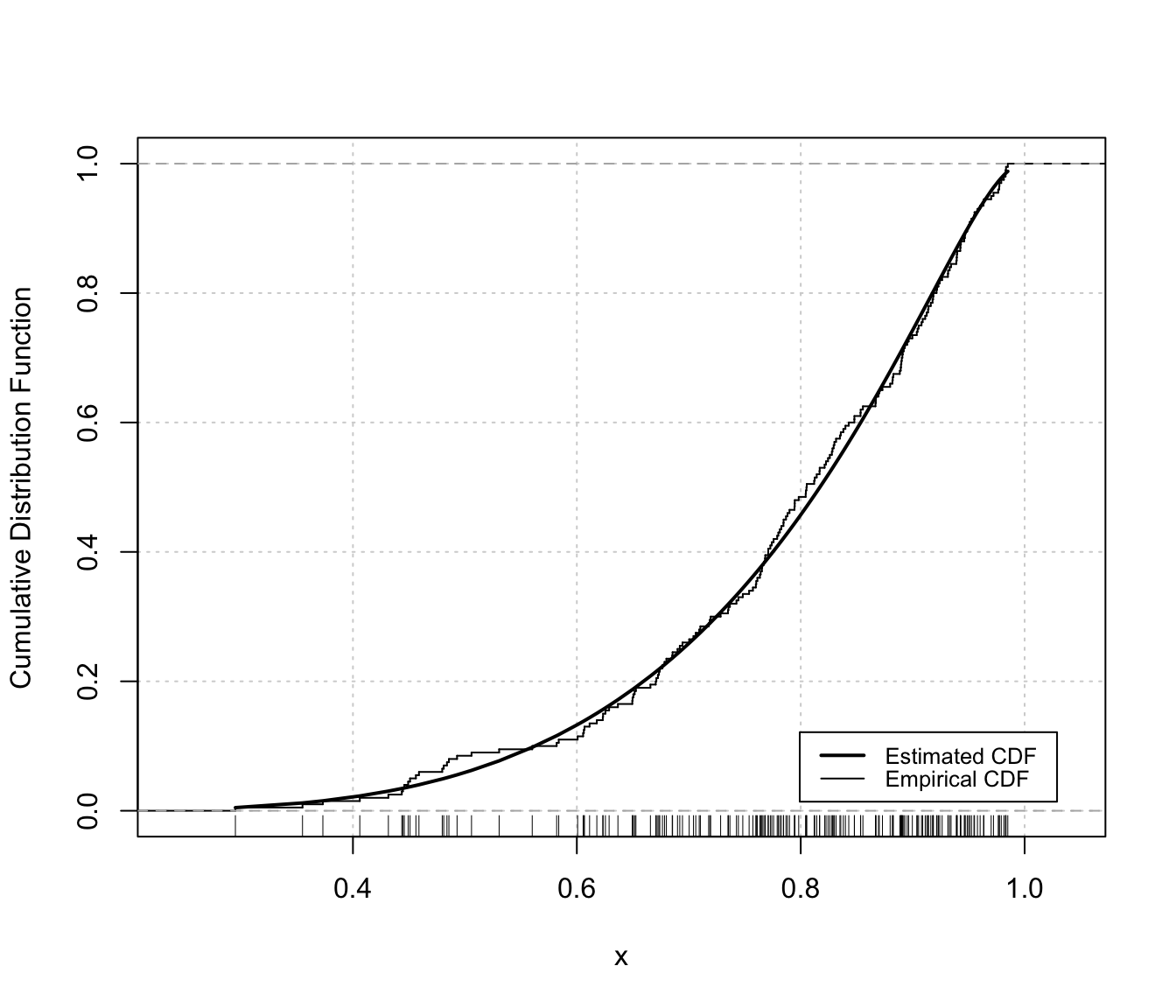
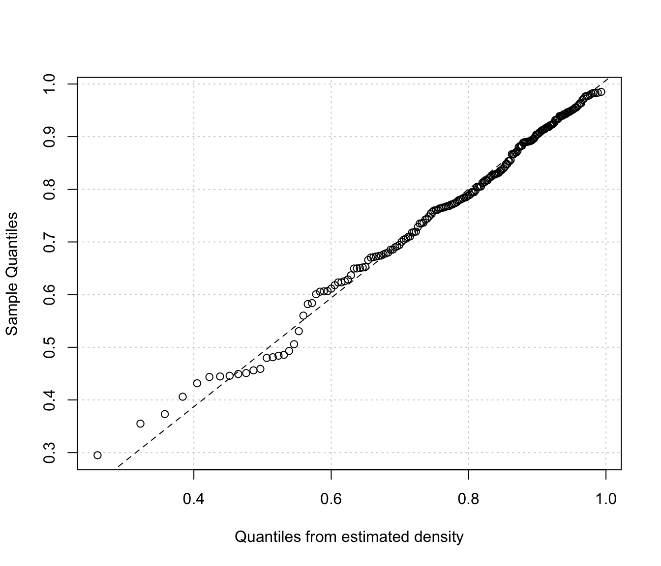
Diagnostic plots for density estimation of bounded data via transformation-based approach of Gaussian mixtures. Only available for the one-dimensional case.

The two diagnostic plots for density estimation in the one-dimensional case are discussed in Loader (1999, pp- 87-90).

Usage

cdfDensityBounded(object, data, ngrid = 100, ...)

quantileDensityBounded(object, p, ...)

densityMclustBounded.diagnostic(
  object,
  type = c("cdf", "qq"),
  col = c("black", "black"),
  lwd = c(2, 1),
  lty = c(1, 1),
  legend = TRUE,
  grid = TRUE,
  ...
)

Arguments

object

An object of class 'mclustDensityBounded' obtained from a call to densityMclustBounded() function.

data

A numeric vector of evaluation points.

ngrid

The number of points in a regular grid to be used as evaluation points if no data are provided.

...

Additional arguments.

p

A numeric vector of probabilities corresponding to quantiles.

type

The type of graph requested:

"cdf" A plot of the estimated CDF versus the empirical distribution function.
"qq" A Q-Q plot of sample quantiles versus the quantiles obtained from the inverse of the estimated cdf.

col

A pair of values for the color to be used for plotting, respectively, the estimated CDF and the empirical cdf.

lwd

A pair of values for the line width to be used for plotting, respectively, the estimated CDF and the empirical cdf.

lty

A pair of values for the line type to be used for plotting, respectively, the estimated CDF and the empirical cdf.

legend

A logical indicating if a legend must be added to the plot of fitted CDF vs the empirical CDF.

grid

A logical indicating if a grid() should be added to the plot.

Value

cdfDensityBounded() returns a list of x and y values providing, respectively, the evaluation points and the estimated cdf.

quantileDensityBounded() returns a vector of quantiles.

No return value, called for side effects.

Details

The cdf is evaluated at points given by the optional argument data. If not provided, a regular grid of length ngrid for the evaluation points is used.

The quantiles are computed using bisection linear search algorithm.

References

Loader C. (1999), Local Regression and Likelihood. New York, Springer.

Author

Luca Scrucca

Examples

# \donttest{
# univariate case with lower bound
x <- rchisq(200, 3)
dens <- densityMclustBounded(x, lbound = 0)

xgrid <- seq(-2, max(x), length=1000)
cdf <- cdfDensityBounded(dens, xgrid)
str(cdf)
#> List of 2
#>  $ x: num [1:1000] -2 -1.98 -1.97 -1.95 -1.93 ...
#>  $ y: num [1:1000] 0 0 0 0 0 0 0 0 0 0 ...
plot(xgrid, pchisq(xgrid, df = 3), type = "l", xlab = "x", ylab = "CDF")
lines(cdf, col = 4, lwd = 2)


q <- quantileDensityBounded(dens, p = c(0.01, 0.1, 0.5, 0.9, 0.99))
cbind(quantile = q, cdf = cdfDensityBounded(dens, q)$y)
#>         quantile  cdf
#> [1,]  0.07667995 0.01
#> [2,]  0.51927506 0.10
#> [3,]  2.25981319 0.50
#> [4,]  6.39193414 0.90
#> [5,] 12.48185916 0.99
plot(cdf, type = "l", col = 4, xlab = "x", ylab = "CDF")
points(q, cdfDensityBounded(dens, q)$y, pch = 19, col = 4)


# univariate case with lower & upper bounds
x <- rbeta(200, 5, 1.5)
dens <- densityMclustBounded(x, lbound = 0, ubound = 1)

xgrid <- seq(-0.1, 1.1, length=1000)
cdf <- cdfDensityBounded(dens, xgrid)
str(cdf)
#> List of 2
#>  $ x: num [1:1000] -0.1 -0.0988 -0.0976 -0.0964 -0.0952 ...
#>  $ y: num [1:1000] 0 0 0 0 0 0 0 0 0 0 ...
plot(xgrid, pbeta(xgrid, 5, 1.5), type = "l", xlab = "x", ylab = "CDF")
lines(cdf, col = 4, lwd = 2)


q <- quantileDensityBounded(dens, p = c(0.01, 0.1, 0.5, 0.9, 0.99))
cbind(quantile = q, cdf = cdfDensityBounded(dens, q)$y)
#>       quantile  cdf
#> [1,] 0.3568030 0.01
#> [2,] 0.5738889 0.10
#> [3,] 0.8250813 0.50
#> [4,] 0.9550278 0.90
#> [5,] 0.9895724 0.99
plot(cdf, type = "l", col = 4, xlab = "x", ylab = "CDF")
points(q, cdfDensityBounded(dens, q)$y, pch = 19, col = 4)

# }

# \donttest{
# univariate case with lower bound
x <- rchisq(200, 3)
dens <- densityMclustBounded(x, lbound = 0)
plot(dens, x, what = "diagnostic")


# or
densityMclustBounded.diagnostic(dens, type = "cdf")

densityMclustBounded.diagnostic(dens, type = "qq")


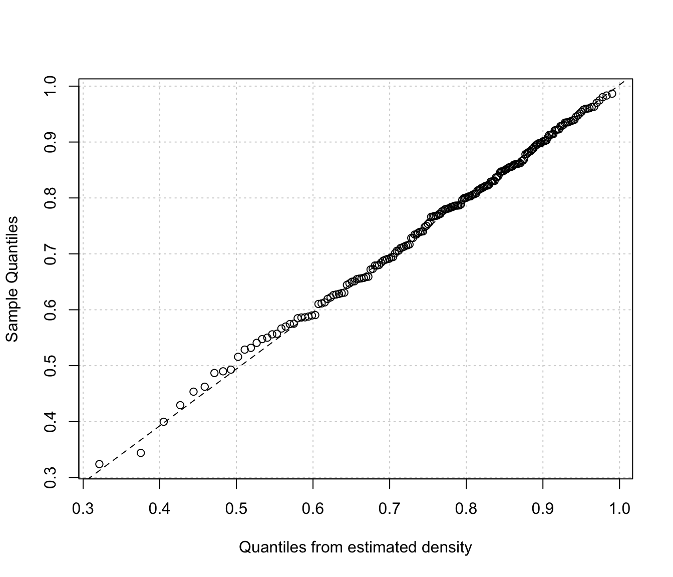# univariate case with lower & upper bounds
x <- rbeta(200, 5, 1.5)
dens <- densityMclustBounded(x, lbound = 0, ubound = 1)
plot(dens, x, what = "diagnostic")


# or
densityMclustBounded.diagnostic(dens, type = "cdf")

densityMclustBounded.diagnostic(dens, type = "qq")

# }