Model-based mixture density estimation for bounded data

Compute density estimation for univariate and multivariate bounded data based on Gaussian finite mixture models estimated by densityMclustBounded.

Usage

# S3 method for densityMclustBounded
predict(object, newdata, 
        what = c("dens", "cdens", "z"), 
        logarithm = FALSE, ...)

Arguments

object: An object of class "densityMclustBounded" resulting from a call to densityMclustBounded.
newdata: A numeric vector, matrix, or data frame of observations. If missing the density is computed for the input data obtained from the call to densityMclustBounded.
what: A character string specifying what to retrieve: "dens" returns a vector of values for the mixture density; "cdens" returns a matrix of component densities for each mixture component (along the columns); "z" returns a matrix of component posterior probabilities.
logarithm: A logical value indicating whether or not the logarithm of the densities/probabilities should be returned.
...: Further arguments passed to or from other methods.

Value

Returns a vector or a matrix of values evaluated at newdata depending on the argument what (see above).

Author

Luca Scrucca

References

Scrucca L. (2019) A transformation-based approach to Gaussian mixture density estimation for bounded data. Biometrical Journal, 61:4, 873–888. https://doi.org/10.1002/bimj.201800174

Examples

# \donttest{
y <- sample(0:1, size = 200, replace = TRUE, prob = c(0.6, 0.4))
x <- y*rchisq(200, 3) + (1-y)*rchisq(200, 10)
dens <- densityMclustBounded(x, lbound = 0)
summary(dens)
#> ── Density estimation for bounded data via GMMs ─────────── 
#>            
#> Boundaries:   x
#>       lower   0
#>       upper Inf
#> 
#> Model E (univariate, equal variance) model with 1 component
#> on the transformation scale:
#> 
#>  log-likelihood   n df       BIC       ICL
#>       -594.3442 200  3 -1204.583 -1204.583
#> 
#>                                     x
#> Range-power transformation: 0.3921889
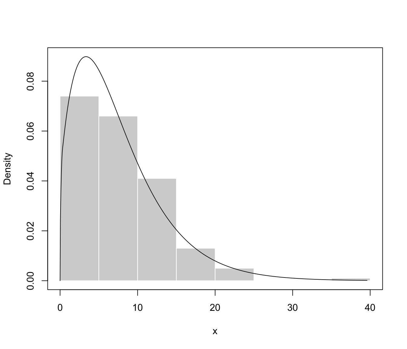
plot(dens, what = "density", data = x, breaks = 11)


xgrid <- seq(0, max(x), length = 201)
densx <- predict(dens, newdata = xgrid, what = "dens")
cdensx <- predict(dens, newdata = xgrid, what = "cdens")
cdensx <- sweep(cdensx, MARGIN = 2, FUN = "*", dens$parameters$pro)
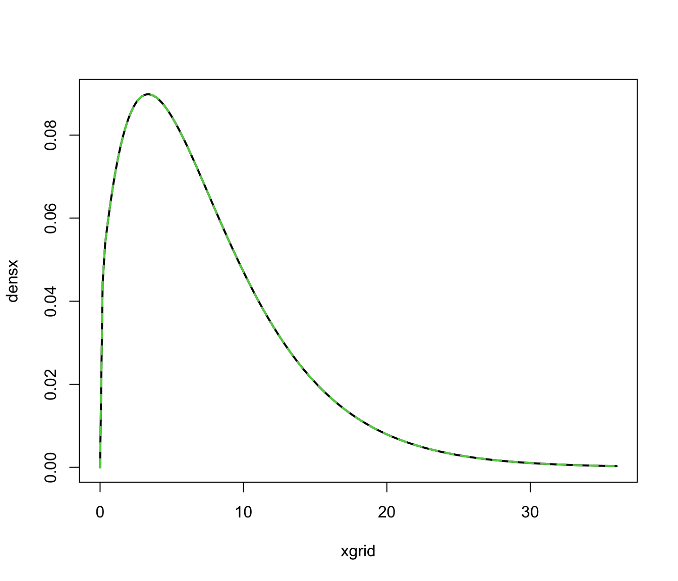
plot(xgrid, densx, type = "l", lwd = 2)
matplot(xgrid, cdensx, type = "l", col = 3:4, lty = 2:3, lwd = 2, add = TRUE)


z <- predict(dens, newdata = xgrid, what = "z")
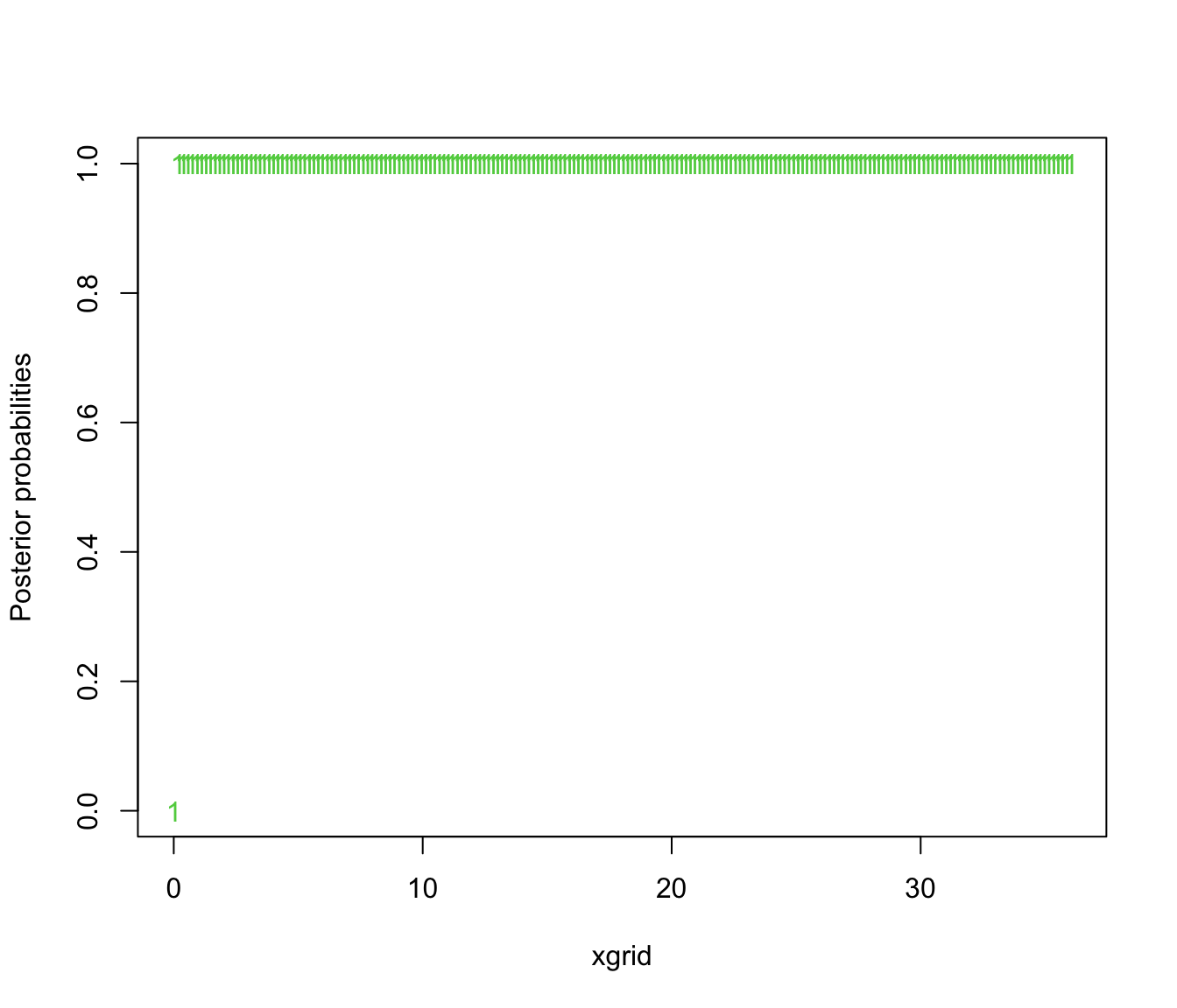
matplot(xgrid, z, col = 3:4, lty = 2:3, lwd = 2, ylab = "Posterior probabilities")

# }