A quick tour of mixggm
Luca Scrucca, Michael Fop, T. Brendan Murphy
19 Nov 2026
mixgmm.RmdIntroduction
The mixggm package implements mixtures of Gaussian graphical models for model-based clustering with sparse covariance and concentration matrices. Estimation of a mixture of Gaussian covariance or concentration graph models using structural-EM algorithm. The mixture model selected is the optimal model according to BIC.
This document gives a quick tour of mixgmm (version
1.2) functionalities. It was written in R Markdown, using the knitr package for
production. See help(package="mixggm") for further details
and references provided by citation("mixggm").
library(mixggm)
##            _
##  _ __ ___ (_)_  ____ _  __ _ _ __ ___
## | '_ ` _ \| \ \/ / _` |/ _` | '_ ` _ \    Mixtures of Gaussian
## | | | | | | |>  < (_| | (_| | | | | | |   Graphical Models
## |_| |_| |_|_/_/\_\__, |\__, |_| |_| |_|
##                  |___/ |___/              Version 1.2
## Type 'citation("mixggm")' for citing this R package in publications.
Fit a mixture of concentration graph models
Iris data
data(iris)
mod = mixGGM(iris[,-5], model = "concentration")
summary(mod)
## ── Mixture of Gaussian graphical models ────────────────────
##
## Data dimensions = 150 x 4
## Model           = concentration
## Search          = forward-stepwise
## Penalty         = bic
##
##  Log-likelihood Pen. log-likelihood df       BIC
##       -219.5572           -237.0944 24 -559.3697
##
## Graphs:
## [,,1]
## Sepal.Length ◯ ◉ ◯ ◯
## Sepal.Width  ◉ ◯ ◯ ◯
## Petal.Length ◯ ◯ ◯ ◉
## Petal.Width  ◯ ◯ ◉ ◯
## [,,2]
## Sepal.Length ◯ ◉ ◉ ◉
## Sepal.Width  ◉ ◯ ◯ ◉
## Petal.Length ◉ ◯ ◯ ◉
## Petal.Width  ◉ ◉ ◉ ◯
summary(mod, graphs = TRUE, clusters = TRUE, parameters = TRUE)
## ── Mixture of Gaussian graphical models ────────────────────
##
## Data dimensions = 150 x 4
## Model           = concentration
## Search          = forward-stepwise
## Penalty         = bic
##
##  Log-likelihood Pen. log-likelihood df       BIC
##       -219.5572           -237.0944 24 -559.3697
##
## Graphs:
## [,,1]
## Sepal.Length ◯ ◉ ◯ ◯
## Sepal.Width  ◉ ◯ ◯ ◯
## Petal.Length ◯ ◯ ◯ ◉
## Petal.Width  ◯ ◯ ◉ ◯
## [,,2]
## Sepal.Length ◯ ◉ ◉ ◉
## Sepal.Width  ◉ ◯ ◯ ◉
## Petal.Length ◉ ◯ ◯ ◉
## Petal.Width  ◉ ◉ ◉ ◯
##
## Clustering table:
##   1   2
##  50 100
##
## Mixing probabilities:
## [1] 0.3333302 0.6666698
##
## Means:
##                      1        2
## Sepal.Length 5.0060047 6.261992
## Sepal.Width  3.4280105 2.871997
## Petal.Length 1.4620015 4.905983
## Petal.Width  0.2459995 1.675994
##
## Concentrations:
## [,,1]
##              Sepal.Length Sepal.Width Petal.Length Petal.Width
## Sepal.Length     18.30626   -12.64066      0.00000     0.00000
## Sepal.Width     -12.64066    15.83050      0.00000     0.00000
## Petal.Length      0.00000     0.00000     38.01504   -20.77518
## Petal.Width       0.00000     0.00000    -20.77518   103.23098
## [,,2]
##              Sepal.Length Sepal.Width Petal.Length Petal.Width
## Sepal.Length     8.374171   -2.539852    -6.726653    4.132758
## Sepal.Width     -2.539852   15.048524     0.000000   -4.321578
## Petal.Length    -6.726653    0.000000    10.295677  -10.244138
## Petal.Width      4.132758   -4.321578   -10.244138   20.079760
plot(mod, what = "graph")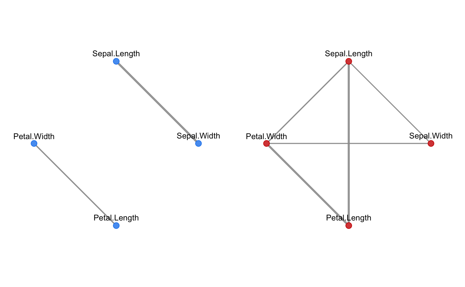
plot(mod, what = "adjacency")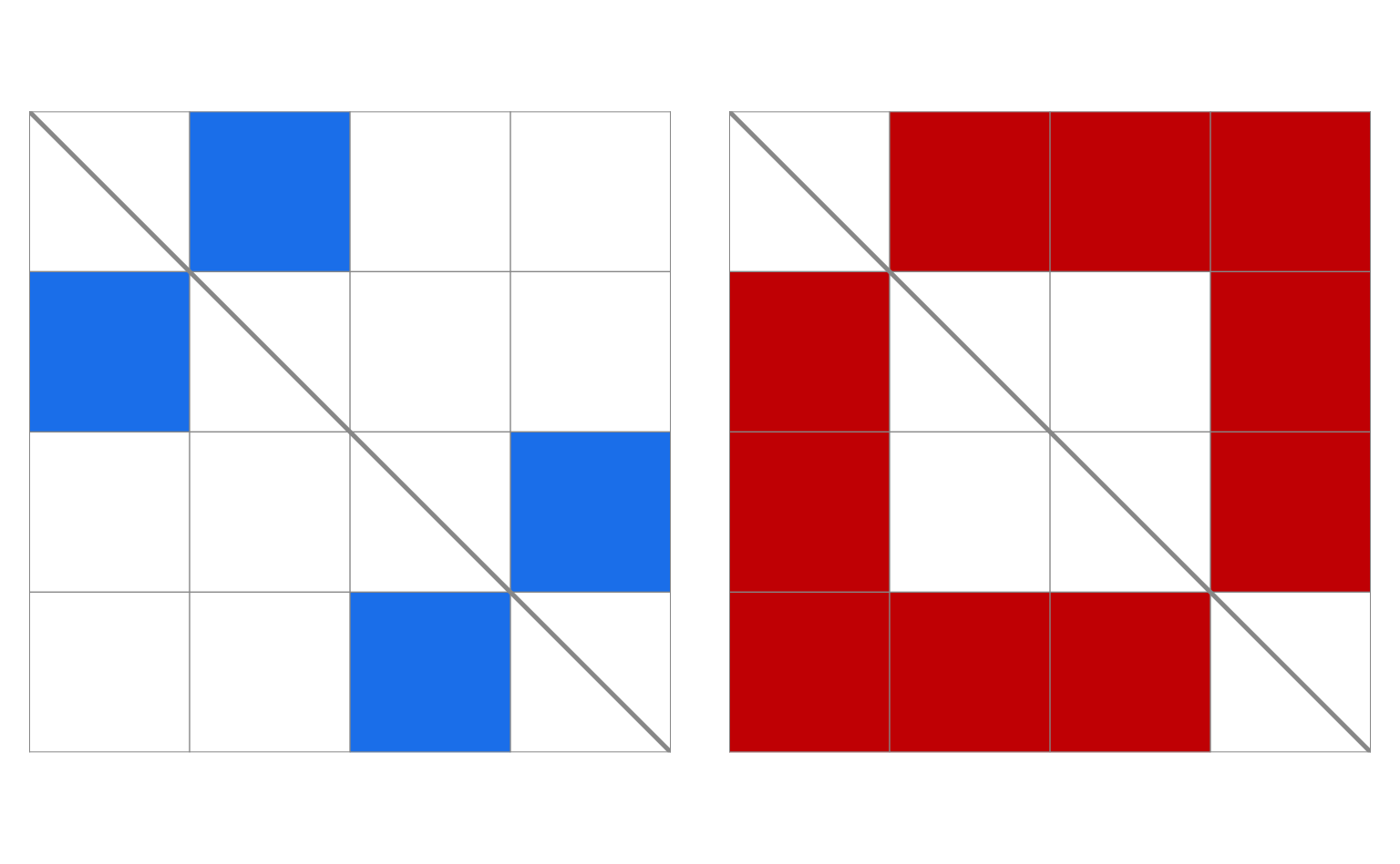
plot(mod, what = "classification")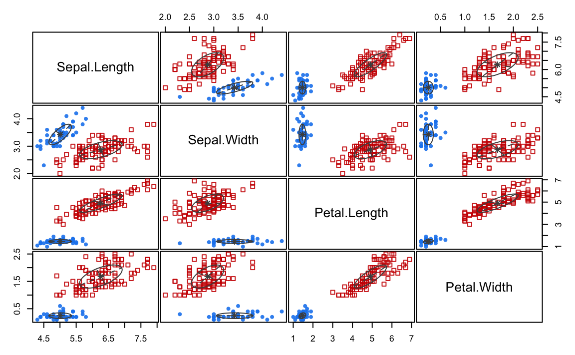
plot(mod, what = "common")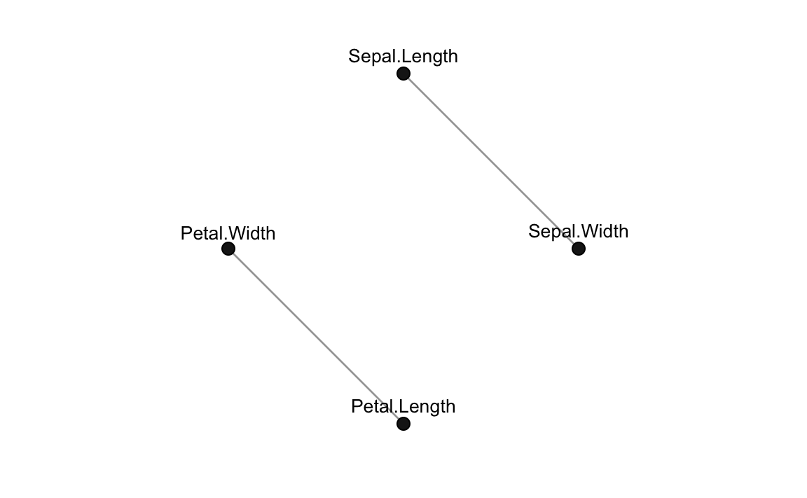
A complex simulated data example
N = 500
V = 20
tau = c(0.3, 0.7)
Nk = rowSums( rmultinom(N, 1, tau) )
class = rep(1:2, Nk)
sigma1 = rWishart(1, V+1, diag(V))[,,1]
mu1 = rep(0, V)
mu2 = rnorm(V, 0.5, 2)
x1 = MASS::mvrnorm(Nk[1], mu1, sigma1)
x2 = matrix(NA, Nk[2], V)
x2[,1] = rnorm(Nk[2])
for(j in 2:V)
  x2[,j] = x2[,j-1] + rnorm(Nk[2], mu2[j], sd = 0.5)
x = rbind(x1, x2)
colnames(x) = paste0("x", 1:ncol(x))
mod = mixGGM(x, K = 1:4, model = "concentration",
             penalty = "ebic", beta = 0.5)
summary(mod)
## ── Mixture of Gaussian graphical models ────────────────────
##
## Data dimensions = 500 x 20
## Model           = concentration
## Search          = forward-stepwise
## Penalty         = ebic
##
##  Log-likelihood Pen. log-likelihood  df       BIC
##       -13384.86           -13818.17 152 -27714.33
##
## Graphs:
## [,,1]
## x1  ◯ ◯ ◯ ◉ ◯ ◯ ◯ ◯ ◯ ◯ ◉ ◯ ◯ ◯ ◯ ◯ ◉ ◉ ◯ ◯
## x2  ◯ ◯ ◯ ◉ ◯ ◯ ◯ ◯ ◯ ◯ ◯ ◉ ◯ ◉ ◉ ◯ ◯ ◉ ◯ ◯
## x3  ◯ ◯ ◯ ◯ ◯ ◯ ◉ ◯ ◯ ◯ ◯ ◉ ◯ ◯ ◉ ◯ ◯ ◯ ◉ ◉
## x4  ◉ ◉ ◯ ◯ ◯ ◯ ◉ ◯ ◯ ◉ ◯ ◉ ◯ ◯ ◯ ◯ ◯ ◉ ◯ ◉
## x5  ◯ ◯ ◯ ◯ ◯ ◯ ◯ ◉ ◯ ◯ ◉ ◯ ◯ ◉ ◯ ◯ ◯ ◯ ◯ ◯
## x6  ◯ ◯ ◯ ◯ ◯ ◯ ◯ ◉ ◉ ◉ ◯ ◯ ◯ ◯ ◯ ◯ ◉ ◯ ◯ ◯
## x7  ◯ ◯ ◉ ◉ ◯ ◯ ◯ ◯ ◯ ◉ ◉ ◯ ◯ ◯ ◉ ◯ ◯ ◯ ◉ ◯
## x8  ◯ ◯ ◯ ◯ ◉ ◉ ◯ ◯ ◯ ◯ ◯ ◯ ◯ ◯ ◯ ◯ ◉ ◯ ◉ ◯
## x9  ◯ ◯ ◯ ◯ ◯ ◉ ◯ ◯ ◯ ◉ ◉ ◯ ◯ ◉ ◯ ◯ ◯ ◯ ◯ ◯
## x10 ◯ ◯ ◯ ◉ ◯ ◉ ◉ ◯ ◉ ◯ ◉ ◯ ◯ ◯ ◉ ◯ ◯ ◉ ◯ ◉
## x11 ◉ ◯ ◯ ◯ ◉ ◯ ◉ ◯ ◉ ◉ ◯ ◯ ◉ ◉ ◯ ◯ ◉ ◉ ◯ ◯
## x12 ◯ ◉ ◉ ◉ ◯ ◯ ◯ ◯ ◯ ◯ ◯ ◯ ◯ ◉ ◯ ◯ ◯ ◉ ◯ ◯
## x13 ◯ ◯ ◯ ◯ ◯ ◯ ◯ ◯ ◯ ◯ ◉ ◯ ◯ ◯ ◯ ◯ ◯ ◯ ◯ ◯
## x14 ◯ ◉ ◯ ◯ ◉ ◯ ◯ ◯ ◉ ◯ ◉ ◉ ◯ ◯ ◯ ◯ ◯ ◯ ◯ ◯
## x15 ◯ ◉ ◉ ◯ ◯ ◯ ◉ ◯ ◯ ◉ ◯ ◯ ◯ ◯ ◯ ◯ ◯ ◯ ◉ ◉
## x16 ◯ ◯ ◯ ◯ ◯ ◯ ◯ ◯ ◯ ◯ ◯ ◯ ◯ ◯ ◯ ◯ ◉ ◉ ◯ ◉
## x17 ◉ ◯ ◯ ◯ ◯ ◉ ◯ ◉ ◯ ◯ ◉ ◯ ◯ ◯ ◯ ◉ ◯ ◯ ◯ ◯
## x18 ◉ ◉ ◯ ◉ ◯ ◯ ◯ ◯ ◯ ◉ ◉ ◉ ◯ ◯ ◯ ◉ ◯ ◯ ◉ ◉
## x19 ◯ ◯ ◉ ◯ ◯ ◯ ◉ ◉ ◯ ◯ ◯ ◯ ◯ ◯ ◉ ◯ ◯ ◉ ◯ ◯
## x20 ◯ ◯ ◉ ◉ ◯ ◯ ◯ ◯ ◯ ◉ ◯ ◯ ◯ ◯ ◉ ◉ ◯ ◉ ◯ ◯
## [,,2]
## x1  ◯ ◉ ◯ ◯ ◯ ◯ ◯ ◯ ◯ ◯ ◯ ◯ ◯ ◯ ◯ ◯ ◯ ◯ ◯ ◯
## x2  ◉ ◯ ◉ ◯ ◯ ◯ ◯ ◯ ◯ ◯ ◯ ◯ ◯ ◯ ◯ ◯ ◯ ◯ ◯ ◯
## x3  ◯ ◉ ◯ ◉ ◯ ◯ ◯ ◯ ◯ ◯ ◯ ◯ ◯ ◯ ◯ ◯ ◯ ◯ ◯ ◯
## x4  ◯ ◯ ◉ ◯ ◉ ◯ ◯ ◯ ◯ ◯ ◯ ◯ ◯ ◯ ◯ ◯ ◯ ◯ ◯ ◯
## x5  ◯ ◯ ◯ ◉ ◯ ◉ ◯ ◯ ◯ ◯ ◯ ◯ ◯ ◯ ◯ ◯ ◯ ◯ ◯ ◯
## x6  ◯ ◯ ◯ ◯ ◉ ◯ ◉ ◯ ◯ ◯ ◯ ◯ ◯ ◯ ◯ ◯ ◯ ◯ ◯ ◯
## x7  ◯ ◯ ◯ ◯ ◯ ◉ ◯ ◉ ◯ ◯ ◯ ◯ ◯ ◯ ◯ ◯ ◯ ◯ ◯ ◯
## x8  ◯ ◯ ◯ ◯ ◯ ◯ ◉ ◯ ◉ ◯ ◯ ◯ ◯ ◯ ◯ ◯ ◯ ◯ ◯ ◯
## x9  ◯ ◯ ◯ ◯ ◯ ◯ ◯ ◉ ◯ ◉ ◯ ◯ ◯ ◯ ◯ ◯ ◯ ◯ ◯ ◯
## x10 ◯ ◯ ◯ ◯ ◯ ◯ ◯ ◯ ◉ ◯ ◉ ◯ ◯ ◯ ◯ ◯ ◯ ◯ ◯ ◯
## x11 ◯ ◯ ◯ ◯ ◯ ◯ ◯ ◯ ◯ ◉ ◯ ◉ ◯ ◯ ◯ ◯ ◯ ◯ ◯ ◯
## x12 ◯ ◯ ◯ ◯ ◯ ◯ ◯ ◯ ◯ ◯ ◉ ◯ ◉ ◯ ◯ ◯ ◯ ◯ ◯ ◯
## x13 ◯ ◯ ◯ ◯ ◯ ◯ ◯ ◯ ◯ ◯ ◯ ◉ ◯ ◉ ◯ ◯ ◯ ◯ ◯ ◯
## x14 ◯ ◯ ◯ ◯ ◯ ◯ ◯ ◯ ◯ ◯ ◯ ◯ ◉ ◯ ◉ ◯ ◯ ◯ ◯ ◯
## x15 ◯ ◯ ◯ ◯ ◯ ◯ ◯ ◯ ◯ ◯ ◯ ◯ ◯ ◉ ◯ ◉ ◯ ◯ ◯ ◯
## x16 ◯ ◯ ◯ ◯ ◯ ◯ ◯ ◯ ◯ ◯ ◯ ◯ ◯ ◯ ◉ ◯ ◉ ◯ ◯ ◯
## x17 ◯ ◯ ◯ ◯ ◯ ◯ ◯ ◯ ◯ ◯ ◯ ◯ ◯ ◯ ◯ ◉ ◯ ◉ ◯ ◯
## x18 ◯ ◯ ◯ ◯ ◯ ◯ ◯ ◯ ◯ ◯ ◯ ◯ ◯ ◯ ◯ ◯ ◉ ◯ ◉ ◯
## x19 ◯ ◯ ◯ ◯ ◯ ◯ ◯ ◯ ◯ ◯ ◯ ◯ ◯ ◯ ◯ ◯ ◯ ◉ ◯ ◉
## x20 ◯ ◯ ◯ ◯ ◯ ◯ ◯ ◯ ◯ ◯ ◯ ◯ ◯ ◯ ◯ ◯ ◯ ◯ ◉ ◯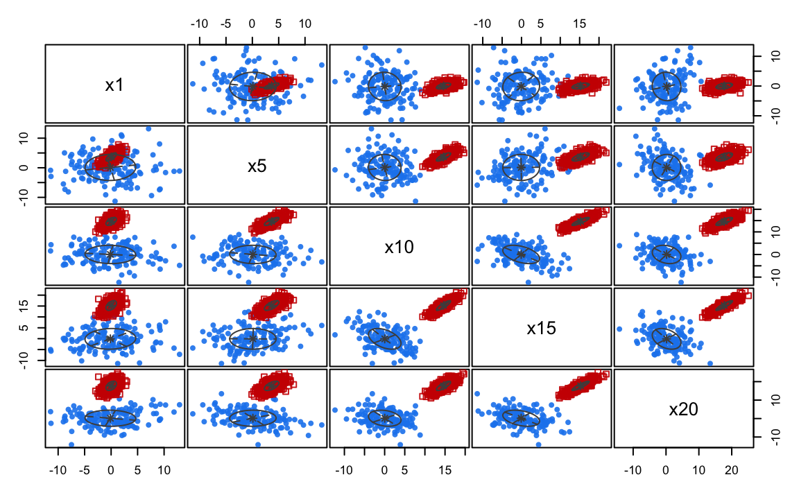
plot(mod, what = "graph")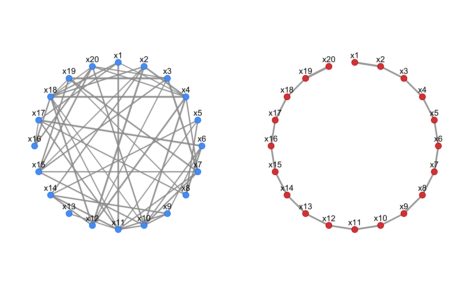
plot(mod, what = "adjacency")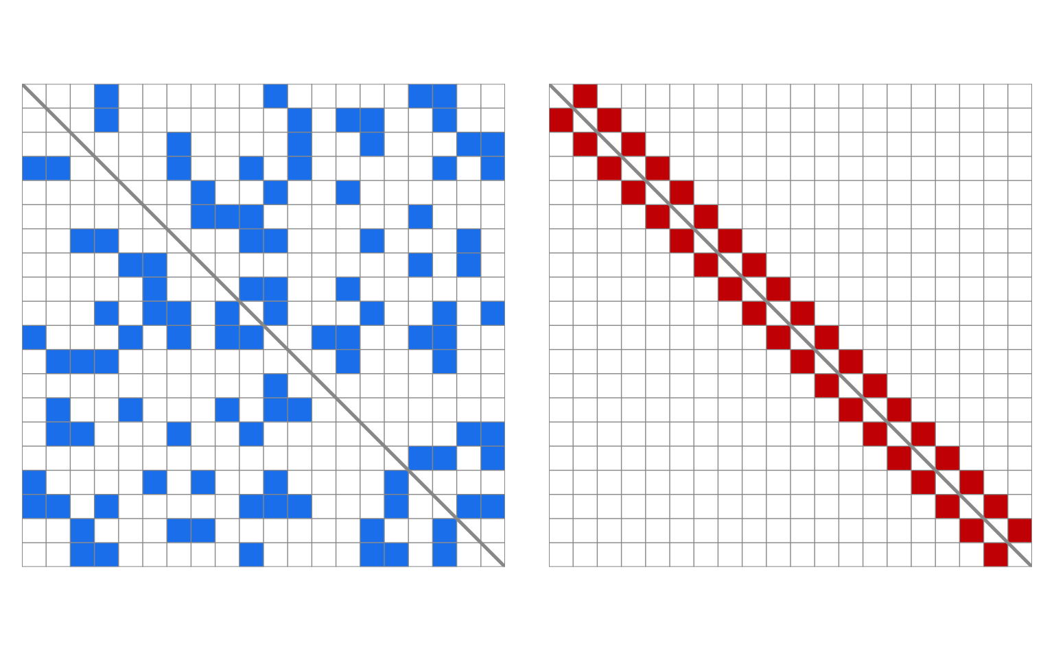
table(class, mod$classification)
##
## class   1   2
##     1 145   0
##     2   0 355
Fit a mixture of covariance graph models
Wine data
data(wine, package = "gclus")
mod = mixGGM(wine[,-1], K = 1:4, model = "covariance",
             penalty = "erdos", beta = 0.01)
summary(mod, graphs = TRUE)
## ── Mixture of Gaussian graphical models ────────────────────
##
## Data dimensions = 178 x 13
## Model           = covariance
## Search          = forward-stepwise
## Penalty         = erdos
##
##  Log-likelihood Pen. log-likelihood  df       BIC
##       -3049.506           -3175.926 107 -6653.463
##
## Graphs:
## [,,1]
## Alcohol         ◯ ◯ ◯ ◯ ◯ ◯ ◯ ◯ ◯ ◯ ◯ ◯ ◯
## Malic           ◯ ◯ ◯ ◯ ◯ ◯ ◯ ◯ ◯ ◯ ◯ ◯ ◯
## Ash             ◯ ◯ ◯ ◯ ◯ ◯ ◯ ◯ ◯ ◯ ◯ ◯ ◯
## Alcalinity      ◯ ◯ ◯ ◯ ◉ ◯ ◯ ◯ ◯ ◯ ◯ ◯ ◯
## Magnesium       ◯ ◯ ◯ ◉ ◯ ◯ ◯ ◯ ◯ ◯ ◯ ◯ ◯
## Phenols         ◯ ◯ ◯ ◯ ◯ ◯ ◉ ◯ ◯ ◉ ◯ ◯ ◯
## Flavanoids      ◯ ◯ ◯ ◯ ◯ ◉ ◯ ◯ ◯ ◉ ◯ ◯ ◯
## Nonflavanoid    ◯ ◯ ◯ ◯ ◯ ◯ ◯ ◯ ◯ ◯ ◯ ◯ ◯
## Proanthocyanins ◯ ◯ ◯ ◯ ◯ ◯ ◯ ◯ ◯ ◯ ◯ ◯ ◯
## Intensity       ◯ ◯ ◯ ◯ ◯ ◉ ◉ ◯ ◯ ◯ ◯ ◯ ◉
## Hue             ◯ ◯ ◯ ◯ ◯ ◯ ◯ ◯ ◯ ◯ ◯ ◯ ◯
## OD280           ◯ ◯ ◯ ◯ ◯ ◯ ◯ ◯ ◯ ◯ ◯ ◯ ◯
## Proline         ◯ ◯ ◯ ◯ ◯ ◯ ◯ ◯ ◯ ◉ ◯ ◯ ◯
## [,,2]
## Alcohol         ◯ ◯ ◯ ◯ ◯ ◯ ◯ ◯ ◯ ◉ ◯ ◯ ◯
## Malic           ◯ ◯ ◯ ◯ ◯ ◯ ◯ ◯ ◯ ◯ ◯ ◯ ◯
## Ash             ◯ ◯ ◯ ◉ ◯ ◯ ◯ ◯ ◯ ◯ ◯ ◯ ◯
## Alcalinity      ◯ ◯ ◉ ◯ ◯ ◯ ◯ ◯ ◯ ◯ ◯ ◯ ◯
## Magnesium       ◯ ◯ ◯ ◯ ◯ ◯ ◉ ◉ ◉ ◯ ◯ ◯ ◉
## Phenols         ◯ ◯ ◯ ◯ ◯ ◯ ◯ ◉ ◉ ◯ ◯ ◯ ◯
## Flavanoids      ◯ ◯ ◯ ◯ ◉ ◯ ◯ ◉ ◉ ◯ ◯ ◯ ◯
## Nonflavanoid    ◯ ◯ ◯ ◯ ◉ ◉ ◉ ◯ ◯ ◯ ◯ ◯ ◯
## Proanthocyanins ◯ ◯ ◯ ◯ ◉ ◉ ◉ ◯ ◯ ◯ ◯ ◯ ◉
## Intensity       ◉ ◯ ◯ ◯ ◯ ◯ ◯ ◯ ◯ ◯ ◉ ◯ ◯
## Hue             ◯ ◯ ◯ ◯ ◯ ◯ ◯ ◯ ◯ ◉ ◯ ◉ ◯
## OD280           ◯ ◯ ◯ ◯ ◯ ◯ ◯ ◯ ◯ ◯ ◉ ◯ ◯
## Proline         ◯ ◯ ◯ ◯ ◉ ◯ ◯ ◯ ◉ ◯ ◯ ◯ ◯
## [,,3]
## Alcohol         ◯ ◯ ◯ ◯ ◯ ◯ ◯ ◯ ◯ ◯ ◯ ◯ ◯
## Malic           ◯ ◯ ◯ ◯ ◯ ◯ ◯ ◯ ◯ ◯ ◉ ◯ ◯
## Ash             ◯ ◯ ◯ ◉ ◉ ◯ ◯ ◯ ◯ ◯ ◯ ◯ ◯
## Alcalinity      ◯ ◯ ◉ ◯ ◯ ◯ ◯ ◯ ◯ ◯ ◯ ◯ ◯
## Magnesium       ◯ ◯ ◉ ◯ ◯ ◯ ◯ ◯ ◯ ◯ ◯ ◯ ◯
## Phenols         ◯ ◯ ◯ ◯ ◯ ◯ ◉ ◉ ◯ ◯ ◯ ◯ ◯
## Flavanoids      ◯ ◯ ◯ ◯ ◯ ◉ ◯ ◯ ◉ ◉ ◯ ◉ ◯
## Nonflavanoid    ◯ ◯ ◯ ◯ ◯ ◉ ◯ ◯ ◯ ◯ ◯ ◯ ◯
## Proanthocyanins ◯ ◯ ◯ ◯ ◯ ◯ ◉ ◯ ◯ ◯ ◯ ◉ ◯
## Intensity       ◯ ◯ ◯ ◯ ◯ ◯ ◉ ◯ ◯ ◯ ◯ ◯ ◯
## Hue             ◯ ◉ ◯ ◯ ◯ ◯ ◯ ◯ ◯ ◯ ◯ ◯ ◯
## OD280           ◯ ◯ ◯ ◯ ◯ ◯ ◉ ◯ ◉ ◯ ◯ ◯ ◯
## Proline         ◯ ◯ ◯ ◯ ◯ ◯ ◯ ◯ ◯ ◯ ◯ ◯ ◯
plot(mod, what = "graph")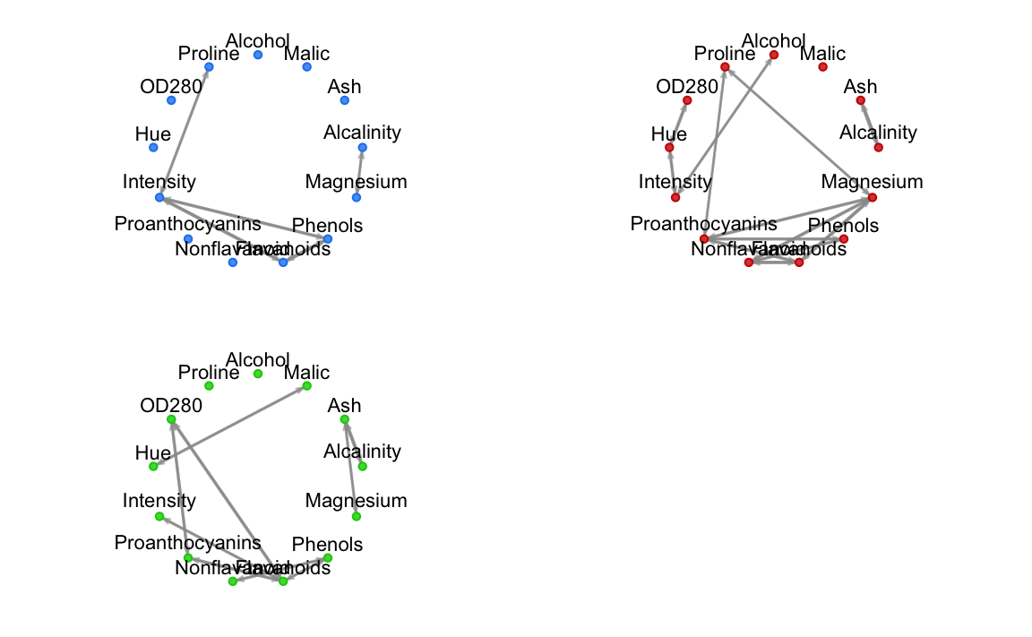
plot(mod, what = "adjacency")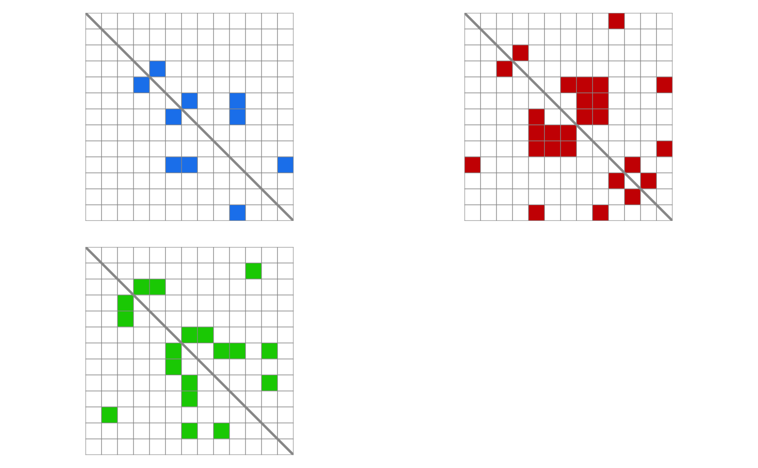
plot(mod, what = "classification", dimens = 1:4)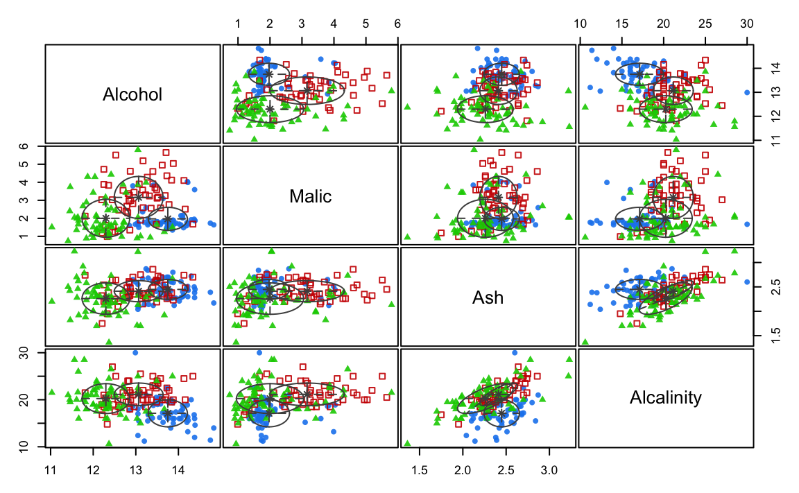
table(wine$Class, mod$classification)
##
##      1  2  3
##   1 57  0  2
##   2  1  5 65
##   3  0 48  0
mclust::adjustedRandIndex(wine$Class, mod$classification)
## [1] 0.8667189
A simple simulated data example
N = 200
tau = c(0.3, 0.7)
Nk = rowSums( rmultinom(N, 1, tau) )
class = rep(1:2, Nk)
sigma1 = diag(2)                          # independent variables
sigma2 = matrix( c(1,0.9,0.9,1), 2,2 )    # correlated variables
mu1 = c(0, 0)
mu2 = c(2, 3)
x = rbind(MASS::mvrnorm(Nk[1], mu1, sigma1),
           MASS::mvrnorm(Nk[2], mu2, sigma2))
colnames(x) = paste0("x", 1:ncol(x))
mod = mixGGM(x, model = "covariance")
summary(mod, graphs = TRUE, parameters = TRUE)
## ── Mixture of Gaussian graphical models ────────────────────
##
## Data dimensions = 200 x 2
## Model           = covariance
## Search          = forward-stepwise
## Penalty         = bic
##
##  Log-likelihood Pen. log-likelihood df      BIC
##       -549.7835           -552.4326 10 -1152.55
##
## Graphs:
## [,,1]
## x1 ◯ ◯
## x2 ◯ ◯
## [,,2]
## x1 ◯ ◉
## x2 ◉ ◯
##
## Mixing probabilities:
## [1] 0.2701669 0.7298331
##
## Means:
##              1        2
## x1 -0.04346726 1.948327
## x2  0.02859949 2.939030
##
## Covariances:
## [,,1]
##          x1        x2
## x1 1.059458 0.0000000
## x2 0.000000 0.9923883
## [,,2]
##          x1        x2
## x1 1.059034 0.9158390
## x2 0.915839 0.9822129
plot(mod, what = "graph")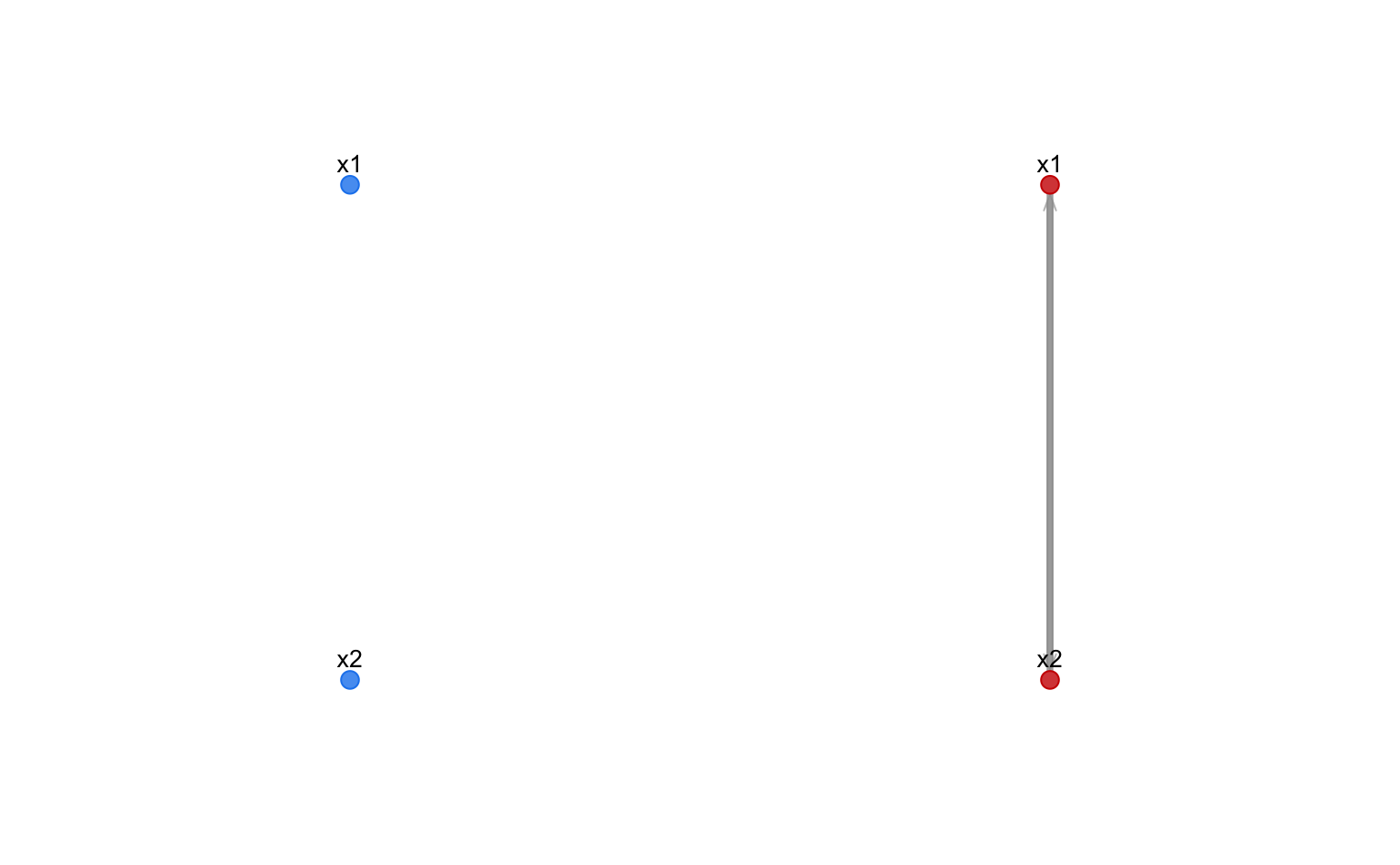
plot(mod, what = "adjacency")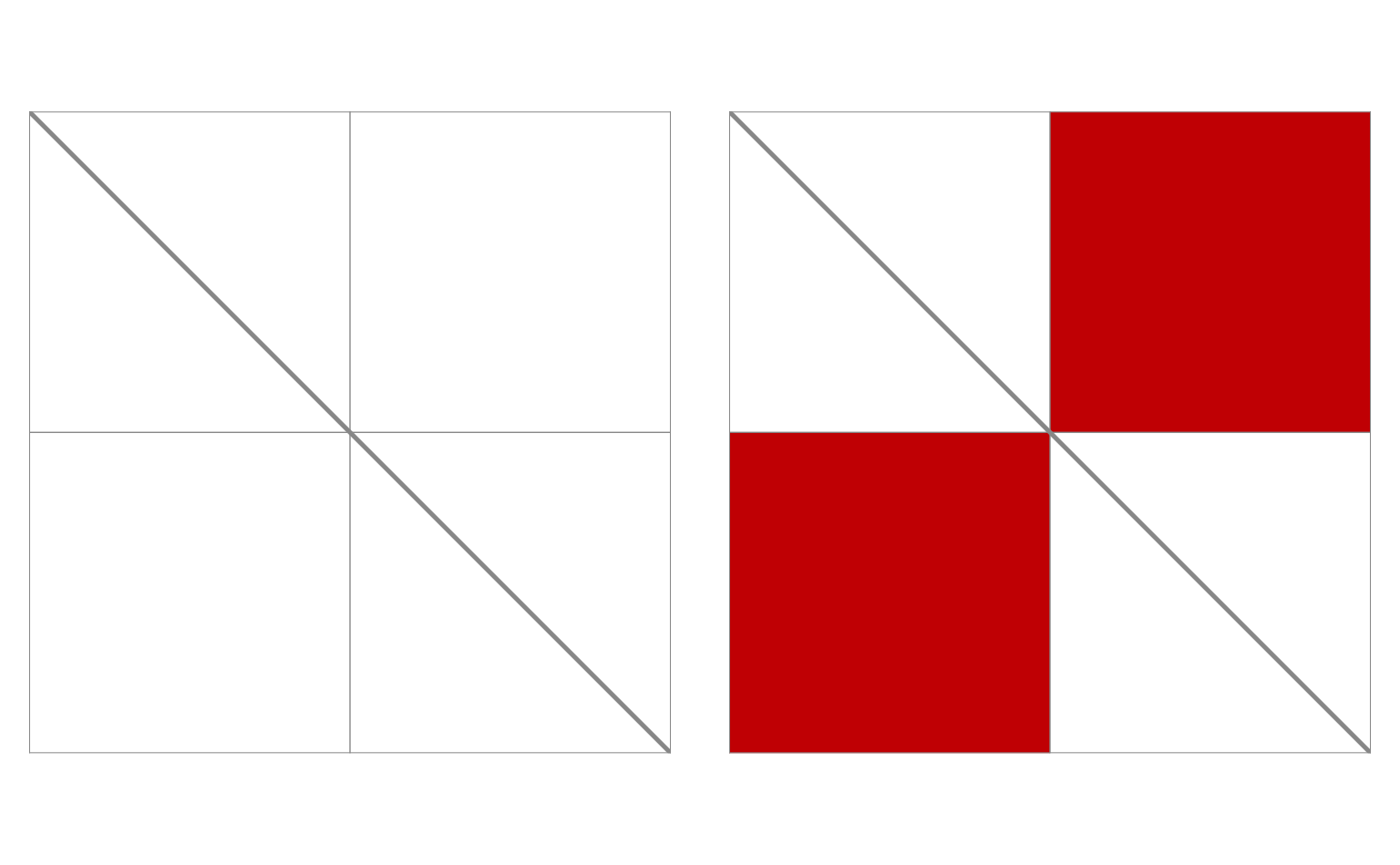
plot(mod, what = "classification")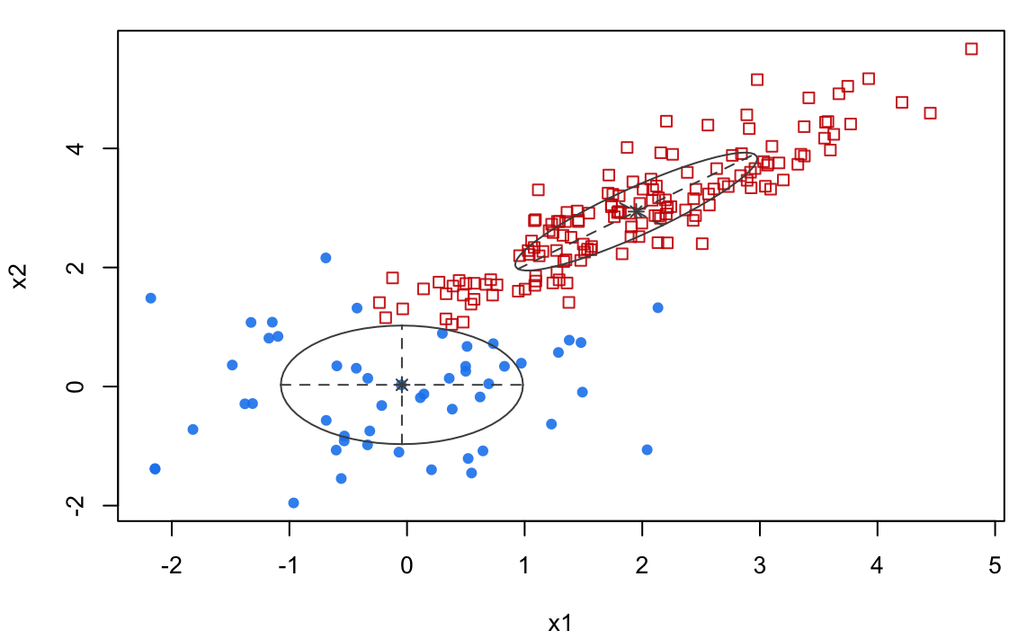
References
Fop M, Murphy TB, Scrucca L (2019). “Model-based clustering with sparse covariance matrices.” Statistics and Computing, 29(4), 791–819. ISSN 1573-1375. doi:10.1007/s11222-018-9838-y.
devtools::session_info()
## ─ Session info ───────────────────────────────────────────────────────────────
##  setting  value
##  version  R version 4.6.2 (2026-10-29)
##  os       macOS Golden Gate 27.2.1
##  system   aarch64, darwin23
##  ui       X11
##  language en
##  collate  en_US.UTF-8
##  ctype    en_US.UTF-8
##  tz       Europe/Rome
##  date     2026-11-19
##  pandoc   3.14 @ /opt/homebrew/bin/ (via rmarkdown)
##  quarto   1.11.9 @ /usr/local/bin/quarto
##
## ─ Packages ───────────────────────────────────────────────────────────────────
##  package        * version  date (UTC) lib source
##  bslib            0.12.0   2026-08-04 [2] CRAN (R 4.6.1)
##  cachem           1.1.0    2024-05-16 [2] CRAN (R 4.6.0)
##  cli              3.6.6    2026-04-09 [2] CRAN (R 4.6.0)
##  coda             0.19-4.1 2024-01-31 [2] CRAN (R 4.6.0)
##  codetools        0.2-20   2024-03-31 [3] CRAN (R 4.6.2)
##  crayon           1.5.3    2024-06-20 [2] CRAN (R 4.6.0)
##  desc             1.4.3    2023-12-10 [2] CRAN (R 4.6.0)
##  devtools         2.5.2    2026-04-30 [2] CRAN (R 4.6.0)
##  digest           0.6.39   2025-11-19 [2] CRAN (R 4.6.0)
##  ellipsis         0.3.3    2026-04-04 [2] CRAN (R 4.6.0)
##  evaluate         1.0.5    2025-08-27 [2] CRAN (R 4.6.0)
##  fastmap          1.2.0    2024-05-15 [2] CRAN (R 4.6.0)
##  foreach          1.5.2    2022-02-02 [2] CRAN (R 4.6.0)
##  fs               2.1.0    2026-04-18 [2] CRAN (R 4.6.0)
##  glue             1.8.1    2026-04-17 [2] CRAN (R 4.6.0)
##  htmltools        0.5.9    2025-12-04 [2] CRAN (R 4.6.0)
##  htmlwidgets      1.6.4    2023-12-06 [2] CRAN (R 4.6.0)
##  iterators        1.0.14   2022-02-05 [2] CRAN (R 4.6.0)
##  jquerylib        0.1.4    2021-04-26 [2] CRAN (R 4.6.0)
##  jsonlite         2.0.0    2025-03-27 [2] CRAN (R 4.6.0)
##  knitr          * 1.52     2026-09-06 [2] CRAN (R 4.6.1)
##  lattice          0.23-1   2026-08-12 [2] CRAN (R 4.6.1)
##  lifecycle        1.0.5    2026-01-08 [2] CRAN (R 4.6.0)
##  magrittr         2.0.5    2026-04-04 [2] CRAN (R 4.6.0)
##  MASS             7.3-66   2026-07-15 [3] CRAN (R 4.6.2)
##  mclust           6.1.4    2026-11-18 [2] CRAN (R 4.6.2)
##  memoise          2.0.1    2021-11-26 [2] CRAN (R 4.6.0)
##  mixggm         * 1.2      2026-11-19 [1] CRAN (R 4.6.2)
##  network          1.20.0   2026-02-07 [2] CRAN (R 4.6.0)
##  otel             0.2.0    2025-08-29 [2] CRAN (R 4.6.0)
##  pillar           1.11.1   2025-09-17 [2] CRAN (R 4.6.0)
##  pkgbuild         1.4.8    2025-05-26 [2] CRAN (R 4.6.0)
##  pkgconfig        2.0.3    2019-09-22 [2] CRAN (R 4.6.0)
##  pkgdown          2.2.1    2026-07-07 [2] CRAN (R 4.6.1)
##  pkgload          1.5.3    2026-06-15 [2] CRAN (R 4.6.0)
##  purrr            1.2.2    2026-04-10 [2] CRAN (R 4.6.0)
##  R6               2.6.1    2025-02-15 [2] CRAN (R 4.6.0)
##  Rcpp             1.1.2    2026-07-05 [2] CRAN (R 4.6.1)
##  rlang            1.3.0    2026-07-05 [2] CRAN (R 4.6.1)
##  rmarkdown        2.32     2026-09-01 [2] CRAN (R 4.6.1)
##  rstudioapi       0.19.0   2026-06-11 [2] CRAN (R 4.6.0)
##  sass             0.4.10   2025-04-11 [2] CRAN (R 4.6.0)
##  sessioninfo      1.2.4    2026-06-04 [2] CRAN (R 4.6.0)
##  statnet.common   4.13.0   2025-12-16 [2] CRAN (R 4.6.0)
##  tibble           3.3.1    2026-01-11 [2] CRAN (R 4.6.0)
##  usethis          3.2.2    2026-09-10 [2] CRAN (R 4.6.1)
##  vctrs            0.7.3    2026-04-11 [2] CRAN (R 4.6.0)
##  xfun             0.62     2026-10-16 [2] CRAN (R 4.6.1)
##  yaml             2.3.12   2025-12-10 [2] CRAN (R 4.6.0)
##
##  [1] /private/var/folders/fw/kxwccvv11xdc27jbny1b8rth0000gn/T/RtmpKTSRQb/temp_libpath51521f970031
##  [2] /Library/Frameworks/R.framework/Rlib
##  [3] /Library/Frameworks/R.framework/Versions/4.6/Resources/library
##  * ── Packages attached to the search path.
##
## ──────────────────────────────────────────────────────────────────────────────