MclustDA discriminant analysis
MclustDA.RdDiscriminant analysis based on Gaussian finite mixture modeling.
Usage
MclustDA(data, class, G = NULL, modelNames = NULL,
         modelType = c("MclustDA", "EDDA"),
         prior = NULL,
         control = emControl(),
         initialization = NULL,
         warn = mclust.options("warn"),
         verbose = interactive(),
         ...)
Arguments
- data
A data frame or matrix giving the training data.
- class
A vector giving the known class labels (either a numerical value or a character string) for the observations in the training data.
- G
An integer vector specifying the numbers of mixture components (clusters) for which the BIC is to be calculated within each class. The default is
G = 1:5.
A different set of mixture components for each class can be specified by providing this argument with a list of integers for each class. See the examples below.- modelNames
A vector of character strings indicating the models to be fitted by EM within each class (see the description in
mclustModelNames). A different set of mixture models for each class can be specified by providing this argument with a list of character strings. See the examples below.- modelType
A character string specifying whether the models given in
modelNamesshould fit a different number of mixture components and covariance structures for each class ("MclustDA", the default) or should be constrained to have a single component for each class with the same covariance structure among classes ("EDDA"). See Details section and the examples below.- prior
The default assumes no prior, but this argument allows specification of a conjugate prior on the means and variances through the function
priorControl.- control
A list of control parameters for EM. The defaults are set by the call
emControl().- initialization
A list containing zero or more of the following components:
hcPairsA matrix of merge pairs for hierarchical clustering such as produced by function
hc. The default is to compute a hierarchical clustering tree by applying functionhcwithmodelName = "E"to univariate data andmodelName = "VVV"to multivariate data or a subset as indicated by thesubsetargument. The hierarchical clustering results are used as starting values for EM.subsetA logical or numeric vector specifying a subset of the data to be used in the initial hierarchical clustering phase.
- warn
A logical value indicating whether or not certain warnings (usually related to singularity) should be issued when estimation fails. The default is controlled by
mclust.options.- verbose
A logical controlling if a text progress bar is displayed during the fitting procedure. By default is
TRUEif the session is interactive, andFALSEotherwise.- ...
Further arguments passed to or from other methods.
Value
An object of class 'MclustDA' providing the optimal (according
to BIC) mixture model.
The details of the output components are as follows:
- call
The matched call.
- data
The input data matrix.
- class
The input class labels.
- type
A character string specifying the
modelTypeestimated.- models
A list of
Mclustobjects containing information on fitted model for each class.- n
The total number of observations in the data.
- d
The dimension of the data.
- bic
Optimal BIC value.
- loglik
Log-likelihood for the selected model.
- df
Number of estimated parameters.
Details
The "EDDA" method for discriminant analysis is described in Bensmail and Celeux (1996), while "MclustDA" in Fraley and Raftery (2002).
References
Scrucca L., Fraley C., Murphy T. B. and Raftery A. E. (2023) Model-Based Clustering, Classification, and Density Estimation Using mclust in R. Chapman & Hall/CRC, ISBN: 978-1032234953, https://mclust-org.github.io/book/
Scrucca L., Fop M., Murphy T. B. and Raftery A. E. (2016) mclust 5: clustering, classification and density estimation using Gaussian finite mixture models, The R Journal, 8/1, pp. 289-317.
Fraley C. and Raftery A. E. (2002) Model-based clustering, discriminant analysis and density estimation, Journal of the American Statistical Association, 97/458, pp. 611-631.
Bensmail, H., and Celeux, G. (1996) Regularized Gaussian Discriminant Analysis Through Eigenvalue Decomposition.Journal of the American Statistical Association, 91, 1743-1748.
Examples
odd <- seq(from = 1, to = nrow(iris), by = 2)
even <- odd + 1
X.train <- iris[odd,-5]
Class.train <- iris[odd,5]
X.test <- iris[even,-5]
Class.test <- iris[even,5]
# common EEE covariance structure (which is essentially equivalent to linear discriminant analysis)
irisMclustDA <- MclustDA(X.train, Class.train, modelType = "EDDA", modelNames = "EEE")
summary(irisMclustDA, parameters = TRUE)
#> ------------------------------------------------
#> Gaussian finite mixture model for classification
#> ------------------------------------------------
#>
#> EDDA
#> ------------------------------------------------
#> log-likelihood n df BIC
#> -125.443 75 24 -354.5057
#>
#> Classes n % Model G
#> setosa 25 33.33 EEE 1
#> versicolor 25 33.33 EEE 1
#> virginica 25 33.33 EEE 1
#>
#> Parameter estimates
#> ------------------------------------------------
#> Class prior probabilities:
#> setosa versicolor virginica
#> 0.3333333 0.3333333 0.3333333
#>
#> Class = setosa
#> --------------
#>
#> Means:
#> [,1]
#> Sepal.Length 5.024
#> Sepal.Width 3.480
#> Petal.Length 1.456
#> Petal.Width 0.228
#>
#> Variances:
#> [,,1]
#> Sepal.Length Sepal.Width Petal.Length Petal.Width
#> Sepal.Length 0.26418133 0.06244800 0.15935467 0.03141333
#> Sepal.Width 0.06244800 0.09630933 0.03326933 0.03222400
#> Petal.Length 0.15935467 0.03326933 0.18236800 0.04091733
#> Petal.Width 0.03141333 0.03222400 0.04091733 0.03891200
#>
#> Class = versicolor
#> ------------------
#>
#> Means:
#> [,1]
#> Sepal.Length 5.992
#> Sepal.Width 2.776
#> Petal.Length 4.308
#> Petal.Width 1.352
#>
#> Variances:
#> [,,1]
#> Sepal.Length Sepal.Width Petal.Length Petal.Width
#> Sepal.Length 0.26418133 0.06244800 0.15935467 0.03141333
#> Sepal.Width 0.06244800 0.09630933 0.03326933 0.03222400
#> Petal.Length 0.15935467 0.03326933 0.18236800 0.04091733
#> Petal.Width 0.03141333 0.03222400 0.04091733 0.03891200
#>
#> Class = virginica
#> -----------------
#>
#> Means:
#> [,1]
#> Sepal.Length 6.504
#> Sepal.Width 2.936
#> Petal.Length 5.564
#> Petal.Width 2.076
#>
#> Variances:
#> [,,1]
#> Sepal.Length Sepal.Width Petal.Length Petal.Width
#> Sepal.Length 0.26418133 0.06244800 0.15935467 0.03141333
#> Sepal.Width 0.06244800 0.09630933 0.03326933 0.03222400
#> Petal.Length 0.15935467 0.03326933 0.18236800 0.04091733
#> Petal.Width 0.03141333 0.03222400 0.04091733 0.03891200
#>
#> Training confusion matrix
#> ------------------------------------------------
#> Predicted
#> Classes setosa versicolor virginica
#> setosa 25 0 0
#> versicolor 0 24 1
#> virginica 0 1 24
#>
#> Classification error = 0.0267
#> Brier score = 0.0097
summary(irisMclustDA, newdata = X.test, newclass = Class.test)
#> ------------------------------------------------
#> Gaussian finite mixture model for classification
#> ------------------------------------------------
#>
#> EDDA
#> ------------------------------------------------
#> log-likelihood n df BIC
#> -125.443 75 24 -354.5057
#>
#> Classes n % Model G
#> setosa 25 33.33 EEE 1
#> versicolor 25 33.33 EEE 1
#> virginica 25 33.33 EEE 1
#>
#> Training confusion matrix
#> ------------------------------------------------
#> Predicted
#> Classes setosa versicolor virginica
#> setosa 25 0 0
#> versicolor 0 24 1
#> virginica 0 1 24
#>
#> Classification error = 0.0267
#> Brier score = 0.0097
#>
#> Test confusion matrix
#> ------------------------------------------------
#> Predicted
#> Classes setosa versicolor virginica
#> setosa 25 0 0
#> versicolor 0 24 1
#> virginica 0 2 23
#>
#> Classification error = 0.0400
#> Brier score = 0.0243
# common covariance structure selected by BIC
irisMclustDA <- MclustDA(X.train, Class.train, modelType = "EDDA")
summary(irisMclustDA, parameters = TRUE)
#> ------------------------------------------------
#> Gaussian finite mixture model for classification
#> ------------------------------------------------
#>
#> EDDA
#> ------------------------------------------------
#> log-likelihood n df BIC
#> -87.93758 75 38 -339.9397
#>
#> Classes n % Model G
#> setosa 25 33.33 VEV 1
#> versicolor 25 33.33 VEV 1
#> virginica 25 33.33 VEV 1
#>
#> Parameter estimates
#> ------------------------------------------------
#> Class prior probabilities:
#> setosa versicolor virginica
#> 0.3333333 0.3333333 0.3333333
#>
#> Class = setosa
#> --------------
#>
#> Means:
#> [,1]
#> Sepal.Length 5.024
#> Sepal.Width 3.480
#> Petal.Length 1.456
#> Petal.Width 0.228
#>
#> Variances:
#> [,,1]
#> Sepal.Length Sepal.Width Petal.Length Petal.Width
#> Sepal.Length 0.154450439 0.097646496 0.017347101 0.005327878
#> Sepal.Width 0.097646496 0.105230813 0.004066916 0.005599939
#> Petal.Length 0.017347101 0.004066916 0.041742267 0.003476241
#> Petal.Width 0.005327878 0.005599939 0.003476241 0.006454832
#>
#> Class = versicolor
#> ------------------
#>
#> Means:
#> [,1]
#> Sepal.Length 5.992
#> Sepal.Width 2.776
#> Petal.Length 4.308
#> Petal.Width 1.352
#>
#> Variances:
#> [,,1]
#> Sepal.Length Sepal.Width Petal.Length Petal.Width
#> Sepal.Length 0.26653496 0.06976610 0.17015657 0.04336127
#> Sepal.Width 0.06976610 0.09861066 0.07509657 0.03823057
#> Petal.Length 0.17015657 0.07509657 0.19799871 0.06126251
#> Petal.Width 0.04336127 0.03823057 0.06126251 0.03627058
#>
#> Class = virginica
#> -----------------
#>
#> Means:
#> [,1]
#> Sepal.Length 6.504
#> Sepal.Width 2.936
#> Petal.Length 5.564
#> Petal.Width 2.076
#>
#> Variances:
#> [,,1]
#> Sepal.Length Sepal.Width Petal.Length Petal.Width
#> Sepal.Length 0.37570480 0.025364426 0.280227270 0.03871029
#> Sepal.Width 0.02536443 0.080872957 0.006413281 0.05009229
#> Petal.Length 0.28022727 0.006413281 0.309059434 0.05805268
#> Petal.Width 0.03871029 0.050092291 0.058052679 0.07540425
#>
#> Training confusion matrix
#> ------------------------------------------------
#> Predicted
#> Classes setosa versicolor virginica
#> setosa 25 0 0
#> versicolor 0 24 1
#> virginica 0 0 25
#>
#> Classification error = 0.0133
#> Brier score = 0.0054
summary(irisMclustDA, newdata = X.test, newclass = Class.test)
#> ------------------------------------------------
#> Gaussian finite mixture model for classification
#> ------------------------------------------------
#>
#> EDDA
#> ------------------------------------------------
#> log-likelihood n df BIC
#> -87.93758 75 38 -339.9397
#>
#> Classes n % Model G
#> setosa 25 33.33 VEV 1
#> versicolor 25 33.33 VEV 1
#> virginica 25 33.33 VEV 1
#>
#> Training confusion matrix
#> ------------------------------------------------
#> Predicted
#> Classes setosa versicolor virginica
#> setosa 25 0 0
#> versicolor 0 24 1
#> virginica 0 0 25
#>
#> Classification error = 0.0133
#> Brier score = 0.0054
#>
#> Test confusion matrix
#> ------------------------------------------------
#> Predicted
#> Classes setosa versicolor virginica
#> setosa 25 0 0
#> versicolor 0 24 1
#> virginica 0 2 23
#>
#> Classification error = 0.0400
#> Brier score = 0.0297
# general covariance structure selected by BIC
irisMclustDA <- MclustDA(X.train, Class.train)
summary(irisMclustDA, parameters = TRUE)
#> ------------------------------------------------
#> Gaussian finite mixture model for classification
#> ------------------------------------------------
#>
#> MclustDA
#> ------------------------------------------------
#> log-likelihood n df BIC
#> -71.74193 75 50 -359.3583
#>
#> Classes n % Model G
#> setosa 25 33.33 VEI 2
#> versicolor 25 33.33 VEE 2
#> virginica 25 33.33 XXX 1
#>
#> Parameter estimates
#> ------------------------------------------------
#> Class prior probabilities:
#> setosa versicolor virginica
#> 0.3333333 0.3333333 0.3333333
#>
#> Class = setosa
#> --------------
#>
#> Mixing probabilities: 0.7229143 0.2770857
#>
#> Means:
#> [,1] [,2]
#> Sepal.Length 5.1761949 4.6269248
#> Sepal.Width 3.6366552 3.0712877
#> Petal.Length 1.4777585 1.3992323
#> Petal.Width 0.2441875 0.1857668
#>
#> Variances:
#> [,,1]
#> Sepal.Length Sepal.Width Petal.Length Petal.Width
#> Sepal.Length 0.120728 0.000000 0.00000000 0.000000000
#> Sepal.Width 0.000000 0.046461 0.00000000 0.000000000
#> Petal.Length 0.000000 0.000000 0.04892923 0.000000000
#> Petal.Width 0.000000 0.000000 0.00000000 0.006358681
#> [,,2]
#> Sepal.Length Sepal.Width Petal.Length Petal.Width
#> Sepal.Length 0.03044364 0.00000000 0.00000000 0.000000000
#> Sepal.Width 0.00000000 0.01171594 0.00000000 0.000000000
#> Petal.Length 0.00000000 0.00000000 0.01233835 0.000000000
#> Petal.Width 0.00000000 0.00000000 0.00000000 0.001603451
#>
#> Class = versicolor
#> ------------------
#>
#> Mixing probabilities: 0.2364317 0.7635683
#>
#> Means:
#> [,1] [,2]
#> Sepal.Length 6.736465 5.761483
#> Sepal.Width 3.000982 2.706336
#> Petal.Length 4.669933 4.195931
#> Petal.Width 1.400893 1.336861
#>
#> Variances:
#> [,,1]
#> Sepal.Length Sepal.Width Petal.Length Petal.Width
#> Sepal.Length 0.030012918 0.008262520 0.02533959 0.008673053
#> Sepal.Width 0.008262520 0.020600060 0.01200205 0.008400168
#> Petal.Length 0.025339590 0.012002053 0.03924151 0.013788157
#> Petal.Width 0.008673053 0.008400168 0.01378816 0.007666627
#> [,,2]
#> Sepal.Length Sepal.Width Petal.Length Petal.Width
#> Sepal.Length 0.16630011 0.04578222 0.14040543 0.04805696
#> Sepal.Width 0.04578222 0.11414392 0.06650279 0.04654492
#> Petal.Length 0.14040543 0.06650279 0.21743528 0.07639950
#> Petal.Width 0.04805696 0.04654492 0.07639950 0.04248041
#>
#> Class = virginica
#> -----------------
#>
#> Mixing probabilities: 1
#>
#> Means:
#> [,1]
#> Sepal.Length 6.504
#> Sepal.Width 2.936
#> Petal.Length 5.564
#> Petal.Width 2.076
#>
#> Variances:
#> [,,1]
#> Sepal.Length Sepal.Width Petal.Length Petal.Width
#> Sepal.Length 0.349184 0.019056 0.272144 0.040896
#> Sepal.Width 0.019056 0.079104 0.011296 0.048064
#> Petal.Length 0.272144 0.011296 0.285504 0.049536
#> Petal.Width 0.040896 0.048064 0.049536 0.074624
#>
#> Training confusion matrix
#> ------------------------------------------------
#> Predicted
#> Classes setosa versicolor virginica
#> setosa 25 0 0
#> versicolor 0 25 0
#> virginica 0 0 25
#>
#> Classification error = 0.0000
#> Brier score = 0.0041
summary(irisMclustDA, newdata = X.test, newclass = Class.test)
#> ------------------------------------------------
#> Gaussian finite mixture model for classification
#> ------------------------------------------------
#>
#> MclustDA
#> ------------------------------------------------
#> log-likelihood n df BIC
#> -71.74193 75 50 -359.3583
#>
#> Classes n % Model G
#> setosa 25 33.33 VEI 2
#> versicolor 25 33.33 VEE 2
#> virginica 25 33.33 XXX 1
#>
#> Training confusion matrix
#> ------------------------------------------------
#> Predicted
#> Classes setosa versicolor virginica
#> setosa 25 0 0
#> versicolor 0 25 0
#> virginica 0 0 25
#>
#> Classification error = 0.0000
#> Brier score = 0.0041
#>
#> Test confusion matrix
#> ------------------------------------------------
#> Predicted
#> Classes setosa versicolor virginica
#> setosa 25 0 0
#> versicolor 0 24 1
#> virginica 0 1 24
#>
#> Classification error = 0.0267
#> Brier score = 0.0159
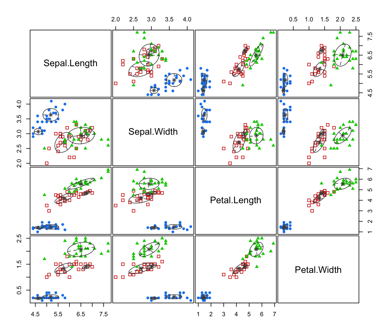
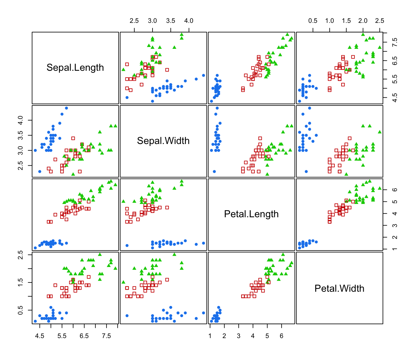
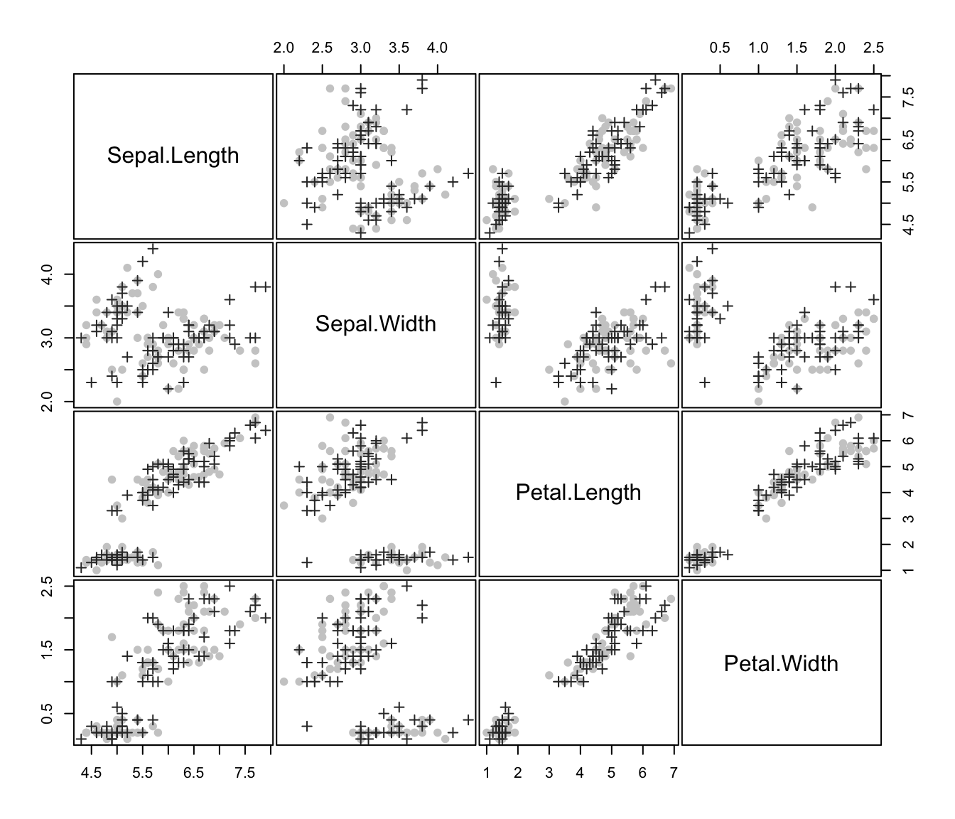
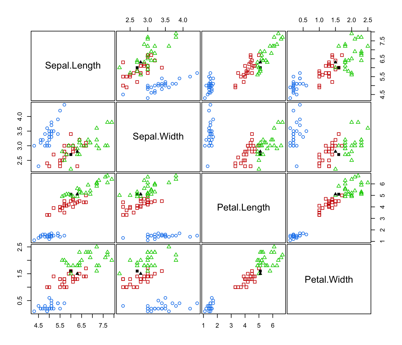
plot(irisMclustDA)
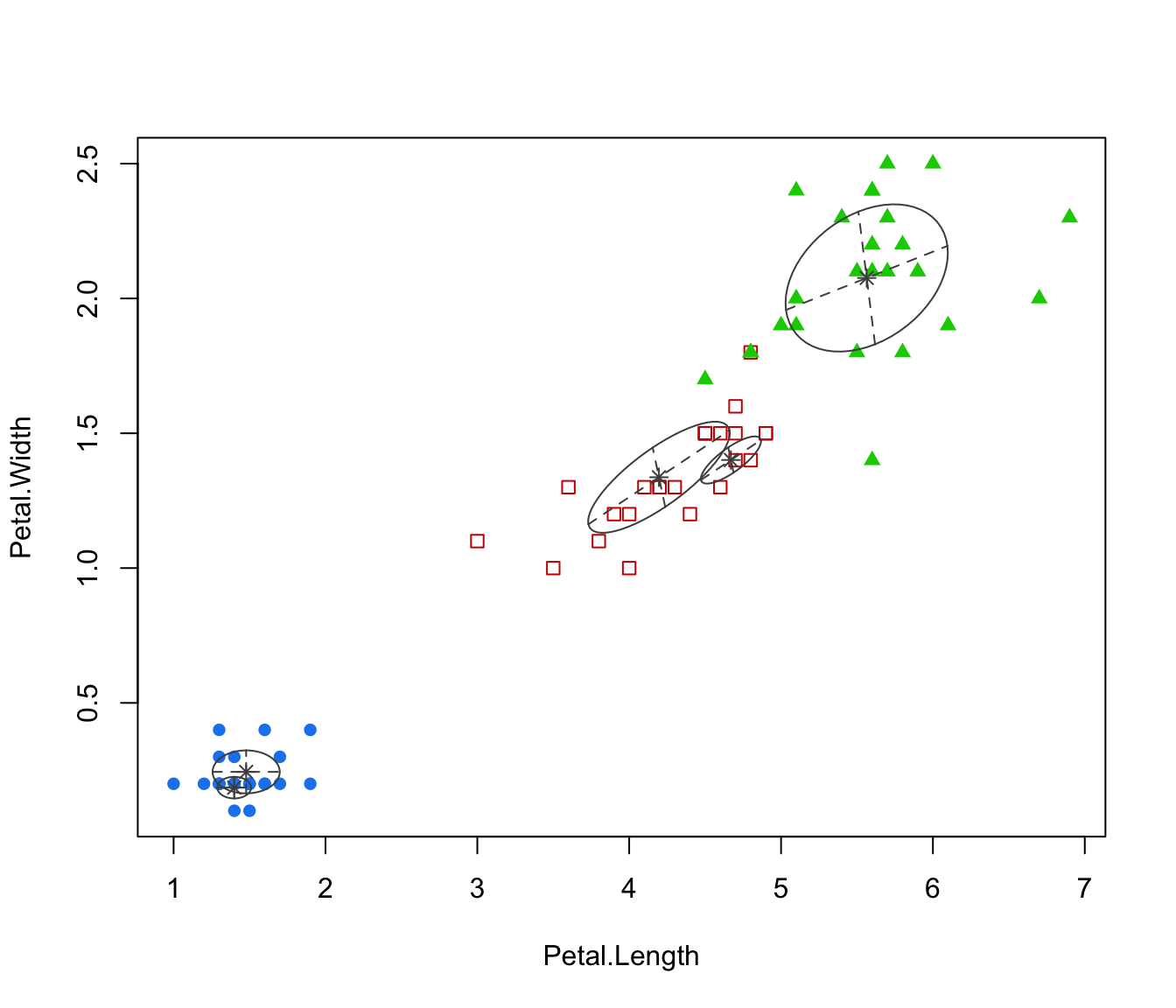
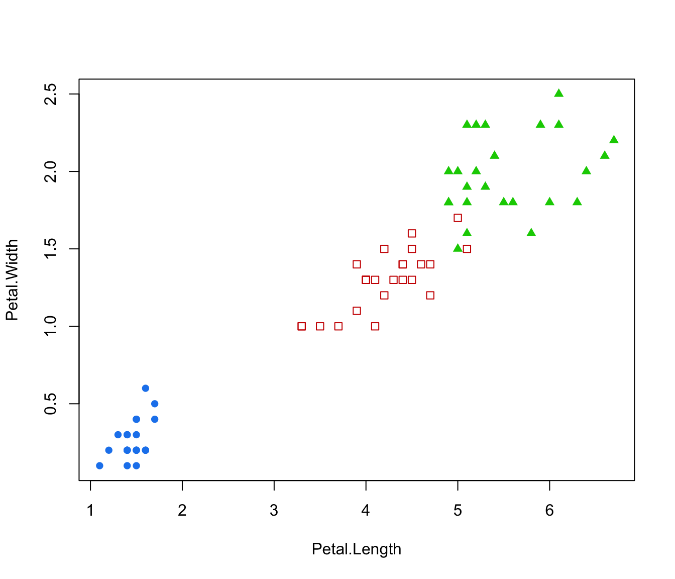
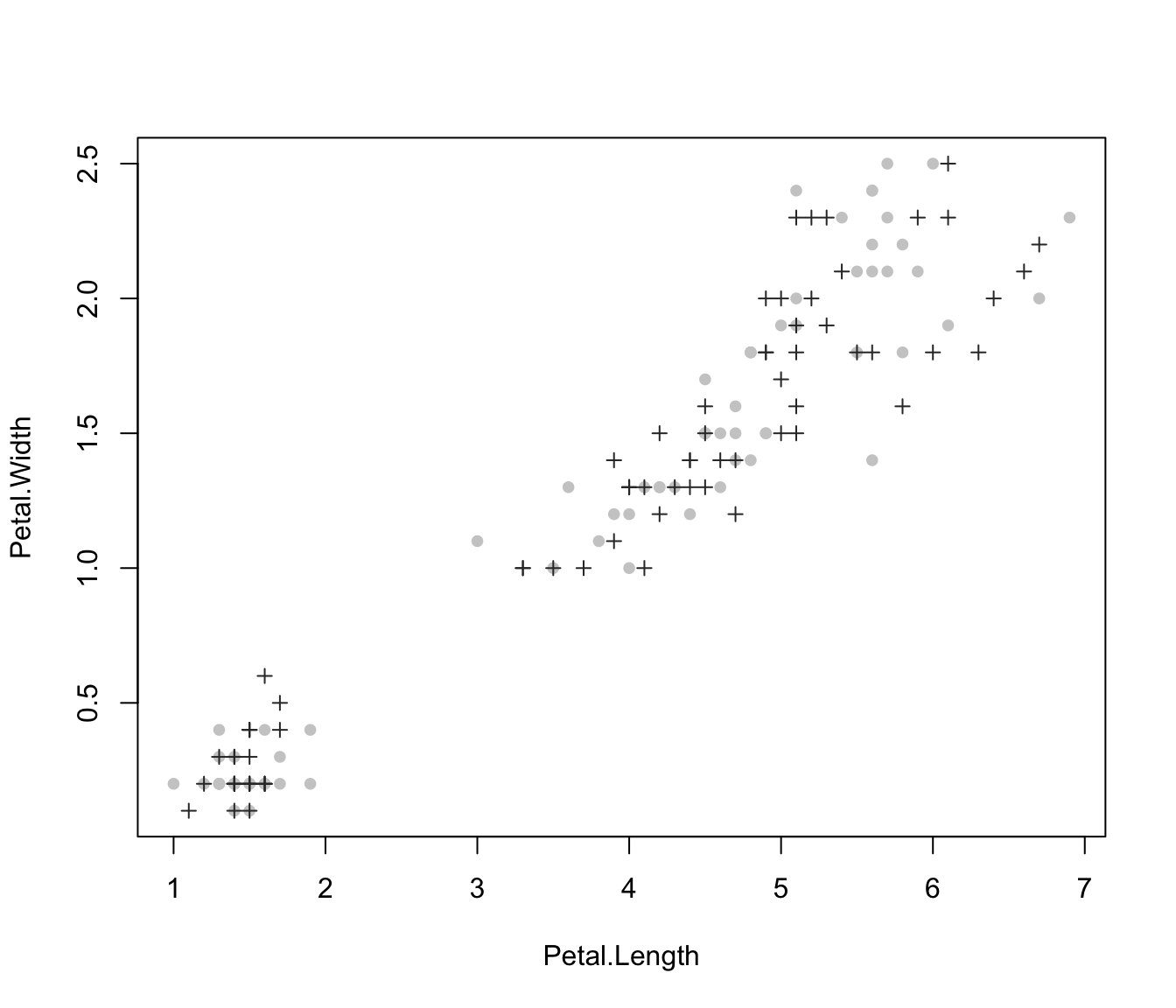
 plot(irisMclustDA, dimens = 3:4)
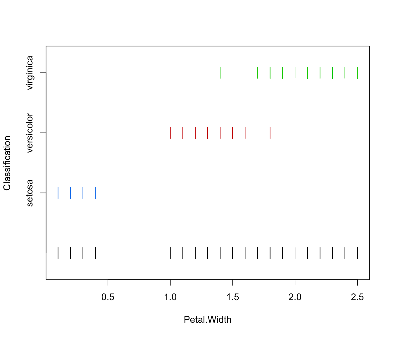
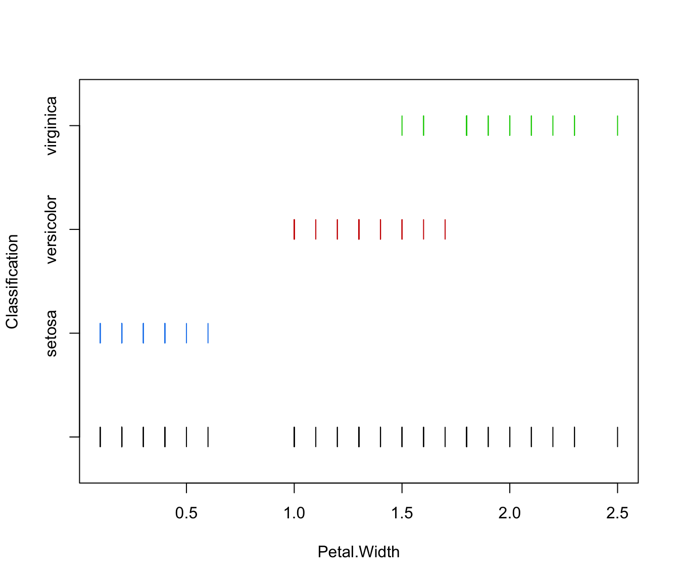
 plot(irisMclustDA, dimens = 4)


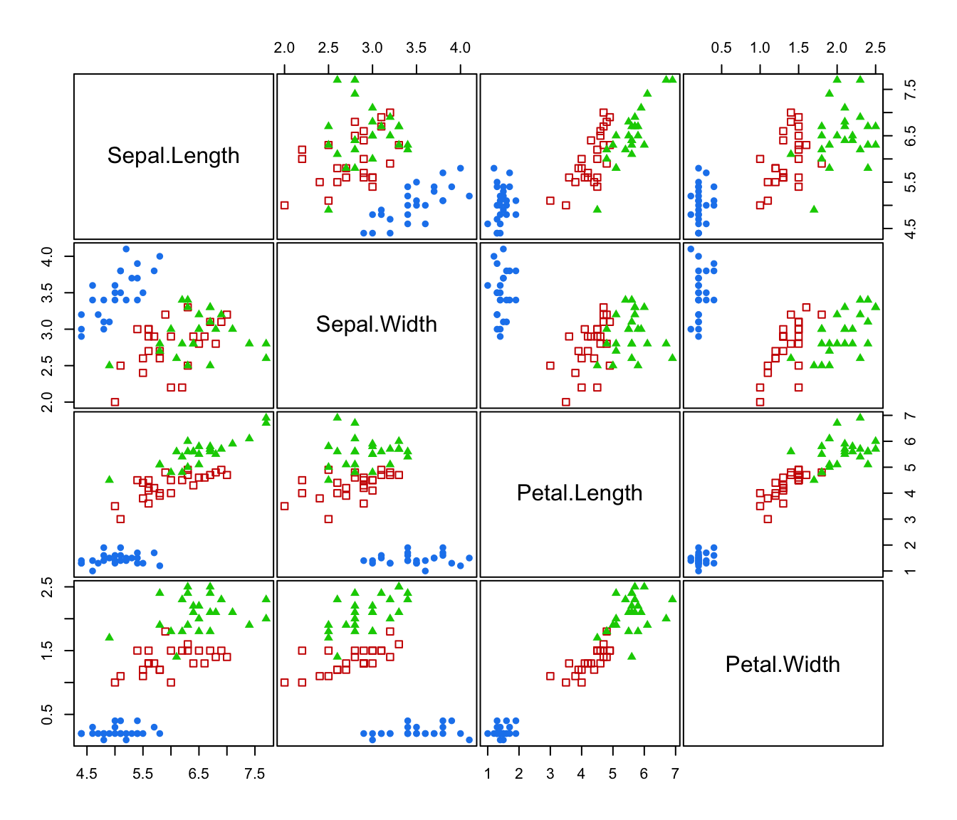
 plot(irisMclustDA, what = "classification")
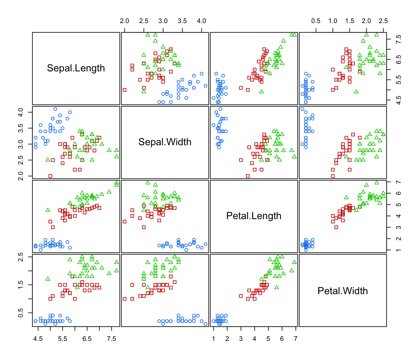
 plot(irisMclustDA, what = "classification", newdata = X.test)
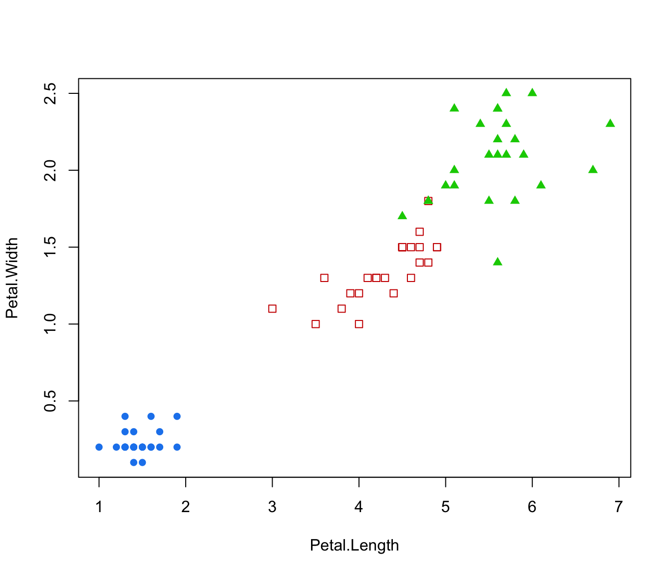
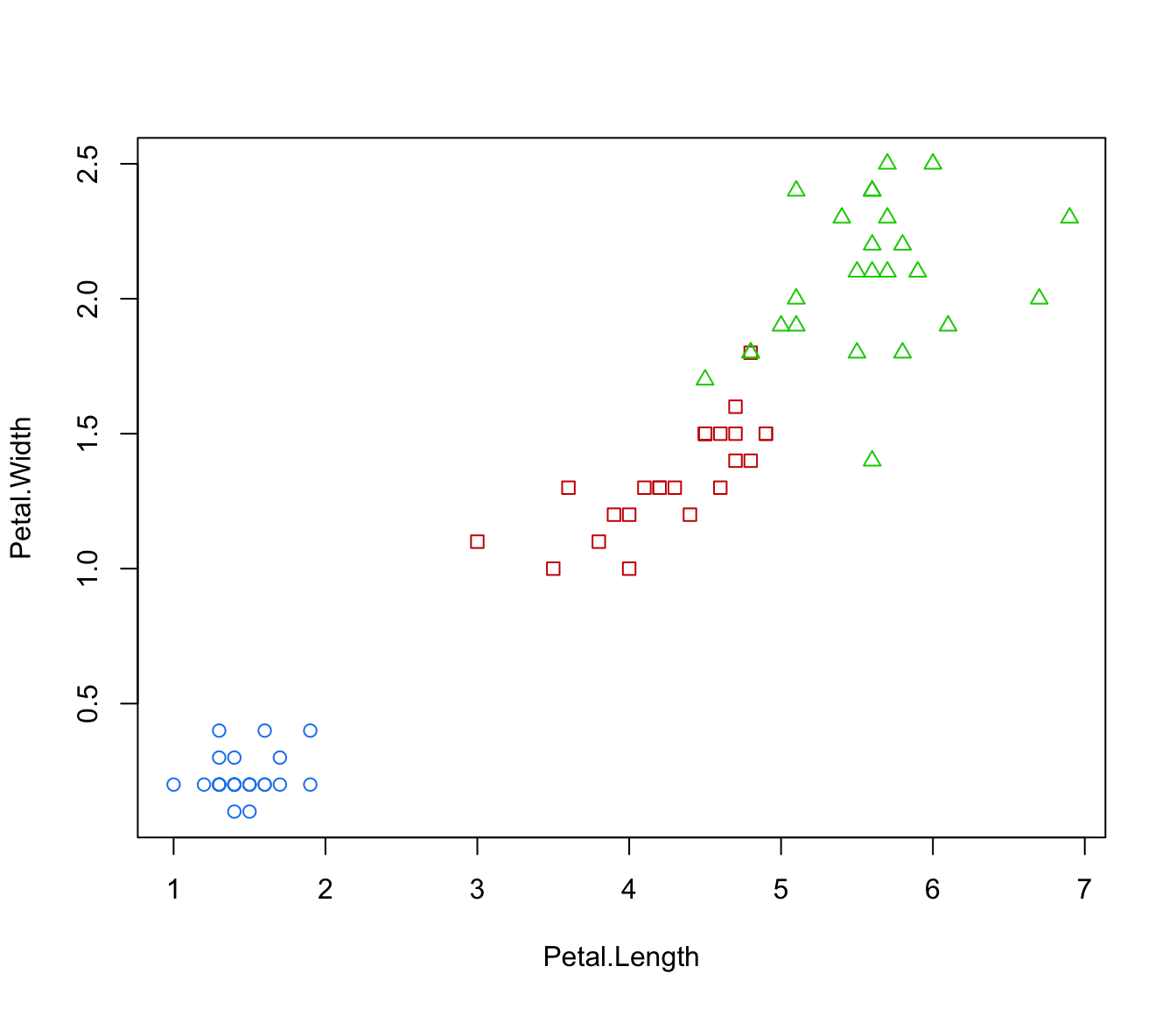
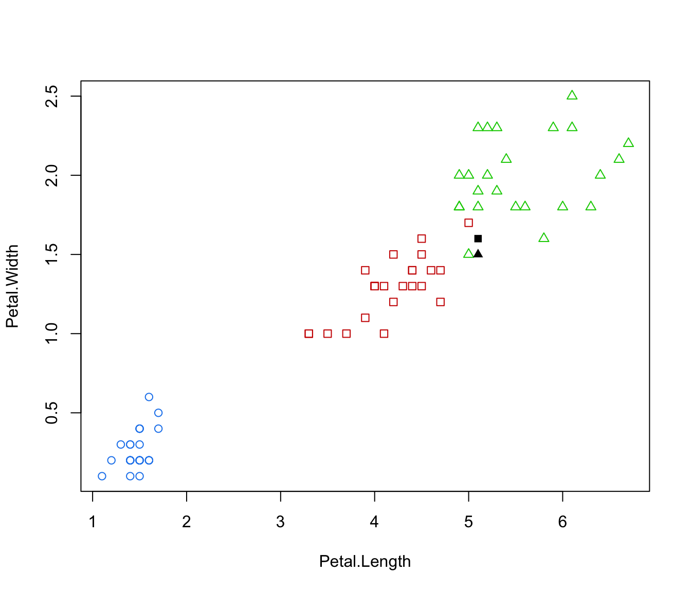
 plot(irisMclustDA, what = "classification", dimens = 3:4)
 plot(irisMclustDA, what = "classification", newdata = X.test, dimens = 3:4)
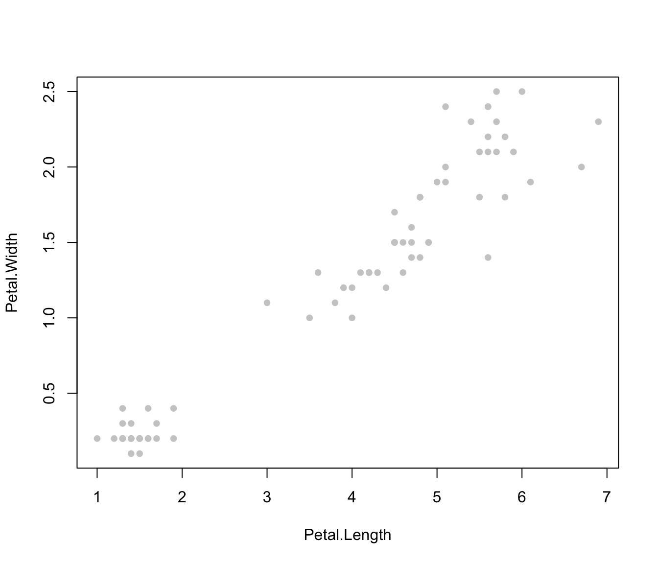
 plot(irisMclustDA, what = "classification", dimens = 4)
 plot(irisMclustDA, what = "classification", dimens = 4, newdata = X.test)
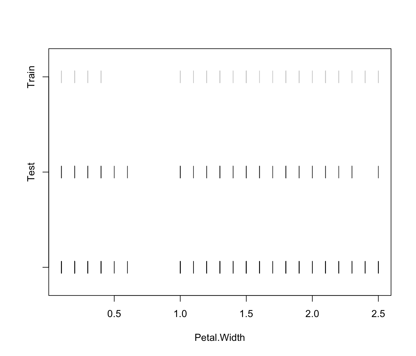
 plot(irisMclustDA, what = "train&test", newdata = X.test)
 plot(irisMclustDA, what = "train&test", newdata = X.test, dimens = 3:4)
 plot(irisMclustDA, what = "train&test", newdata = X.test, dimens = 4)
 plot(irisMclustDA, what = "error")
 plot(irisMclustDA, what = "error", dimens = 3:4)
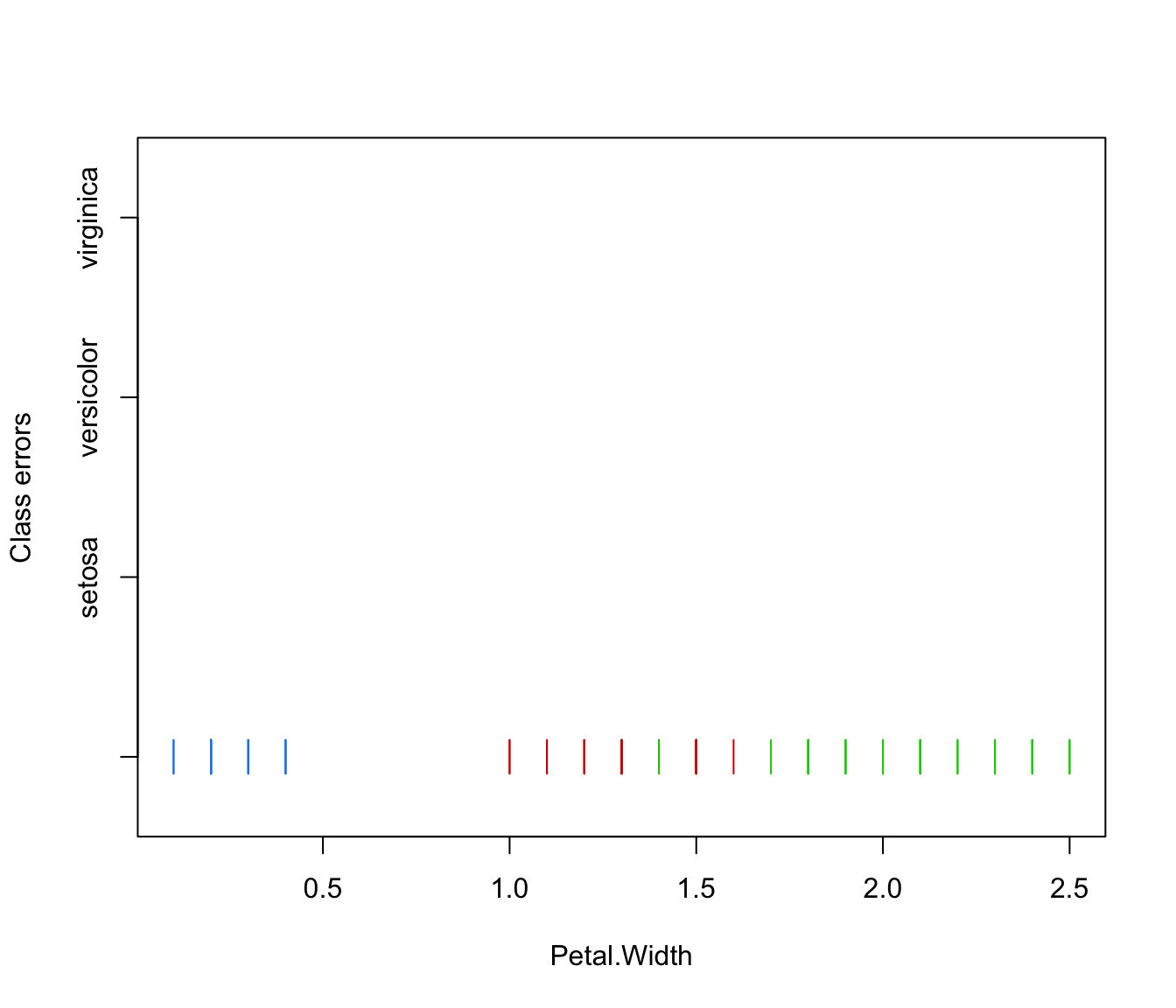
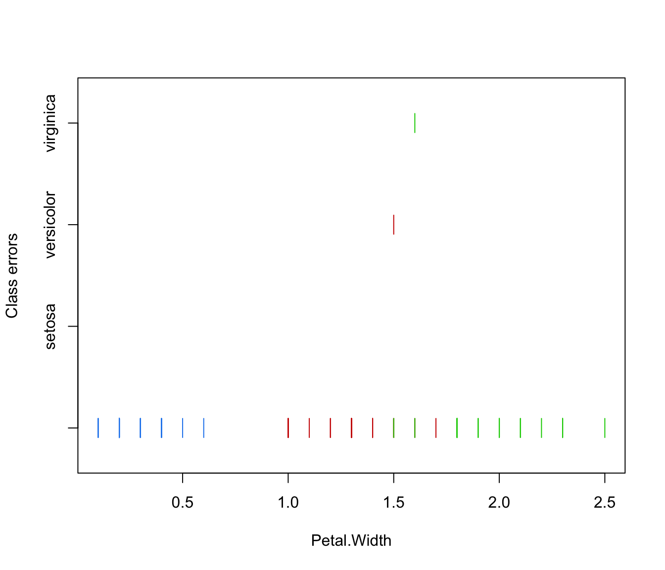
 plot(irisMclustDA, what = "error", dimens = 4)
 plot(irisMclustDA, what = "error", newdata = X.test, newclass = Class.test)
 plot(irisMclustDA, what = "error", newdata = X.test, newclass = Class.test, dimens = 3:4)
 plot(irisMclustDA, what = "error", newdata = X.test, newclass = Class.test, dimens = 4)
 # \donttest{
# simulated 1D data
n <- 250
set.seed(1)
triModal <- c(rnorm(n,-5), rnorm(n,0), rnorm(n,5))
triClass <- c(rep(1,n), rep(2,n), rep(3,n))
odd <- seq(from = 1, to = length(triModal), by = 2)
even <- odd + 1
triMclustDA <- MclustDA(triModal[odd], triClass[odd])
summary(triMclustDA, parameters = TRUE)
#> ------------------------------------------------
#> Gaussian finite mixture model for classification
#> ------------------------------------------------
#>
#> MclustDA
#> ------------------------------------------------
#> log-likelihood n df BIC
#> -942.4306 375 8 -1932.277
#>
#> Classes n % Model G
#> 1 125 33.33 X 1
#> 2 125 33.33 X 1
#> 3 125 33.33 X 1
#>
#> Parameter estimates
#> ------------------------------------------------
#> Class prior probabilities:
#> 1 2 3
#> 0.3333333 0.3333333 0.3333333
#>
#> Class = 1
#> ---------
#>
#> Mixing probabilities: 1
#>
#> Means:
#> [1] -4.951981
#>
#> Variances:
#> [1] 0.8268339
#>
#> Class = 2
#> ---------
#>
#> Mixing probabilities: 1
#>
#> Means:
#> [1] -0.01814707
#>
#> Variances:
#> [1] 1.201987
#>
#> Class = 3
#> ---------
#>
#> Mixing probabilities: 1
#>
#> Means:
#> [1] 4.875429
#>
#> Variances:
#> [1] 1.200321
#>
#> Training confusion matrix
#> ------------------------------------------------
#> Predicted
#> Classes 1 2 3
#> 1 124 1 0
#> 2 0 124 1
#> 3 0 0 125
#>
#> Classification error = 0.0053
#> Brier score = 0.0073
summary(triMclustDA, newdata = triModal[even], newclass = triClass[even])
#> ------------------------------------------------
#> Gaussian finite mixture model for classification
#> ------------------------------------------------
#>
#> MclustDA
#> ------------------------------------------------
#> log-likelihood n df BIC
#> -942.4306 375 8 -1932.277
#>
#> Classes n % Model G
#> 1 125 33.33 X 1
#> 2 125 33.33 X 1
#> 3 125 33.33 X 1
#>
#> Training confusion matrix
#> ------------------------------------------------
#> Predicted
#> Classes 1 2 3
#> 1 124 1 0
#> 2 0 124 1
#> 3 0 0 125
#>
#> Classification error = 0.0053
#> Brier score = 0.0073
#>
#> Test confusion matrix
#> ------------------------------------------------
#> Predicted
#> Classes 1 2 3
#> 1 124 1 0
#> 2 1 122 2
#> 3 0 1 124
#>
#> Classification error = 0.0133
#> Brier score = 0.0089
plot(triMclustDA, what = "scatterplot")
# \donttest{
# simulated 1D data
n <- 250
set.seed(1)
triModal <- c(rnorm(n,-5), rnorm(n,0), rnorm(n,5))
triClass <- c(rep(1,n), rep(2,n), rep(3,n))
odd <- seq(from = 1, to = length(triModal), by = 2)
even <- odd + 1
triMclustDA <- MclustDA(triModal[odd], triClass[odd])
summary(triMclustDA, parameters = TRUE)
#> ------------------------------------------------
#> Gaussian finite mixture model for classification
#> ------------------------------------------------
#>
#> MclustDA
#> ------------------------------------------------
#> log-likelihood n df BIC
#> -942.4306 375 8 -1932.277
#>
#> Classes n % Model G
#> 1 125 33.33 X 1
#> 2 125 33.33 X 1
#> 3 125 33.33 X 1
#>
#> Parameter estimates
#> ------------------------------------------------
#> Class prior probabilities:
#> 1 2 3
#> 0.3333333 0.3333333 0.3333333
#>
#> Class = 1
#> ---------
#>
#> Mixing probabilities: 1
#>
#> Means:
#> [1] -4.951981
#>
#> Variances:
#> [1] 0.8268339
#>
#> Class = 2
#> ---------
#>
#> Mixing probabilities: 1
#>
#> Means:
#> [1] -0.01814707
#>
#> Variances:
#> [1] 1.201987
#>
#> Class = 3
#> ---------
#>
#> Mixing probabilities: 1
#>
#> Means:
#> [1] 4.875429
#>
#> Variances:
#> [1] 1.200321
#>
#> Training confusion matrix
#> ------------------------------------------------
#> Predicted
#> Classes 1 2 3
#> 1 124 1 0
#> 2 0 124 1
#> 3 0 0 125
#>
#> Classification error = 0.0053
#> Brier score = 0.0073
summary(triMclustDA, newdata = triModal[even], newclass = triClass[even])
#> ------------------------------------------------
#> Gaussian finite mixture model for classification
#> ------------------------------------------------
#>
#> MclustDA
#> ------------------------------------------------
#> log-likelihood n df BIC
#> -942.4306 375 8 -1932.277
#>
#> Classes n % Model G
#> 1 125 33.33 X 1
#> 2 125 33.33 X 1
#> 3 125 33.33 X 1
#>
#> Training confusion matrix
#> ------------------------------------------------
#> Predicted
#> Classes 1 2 3
#> 1 124 1 0
#> 2 0 124 1
#> 3 0 0 125
#>
#> Classification error = 0.0053
#> Brier score = 0.0073
#>
#> Test confusion matrix
#> ------------------------------------------------
#> Predicted
#> Classes 1 2 3
#> 1 124 1 0
#> 2 1 122 2
#> 3 0 1 124
#>
#> Classification error = 0.0133
#> Brier score = 0.0089
plot(triMclustDA, what = "scatterplot")
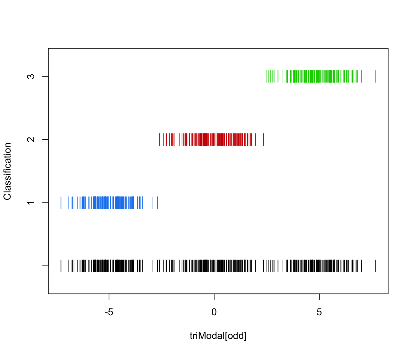
 plot(triMclustDA, what = "classification")
 plot(triMclustDA, what = "classification", newdata = triModal[even])
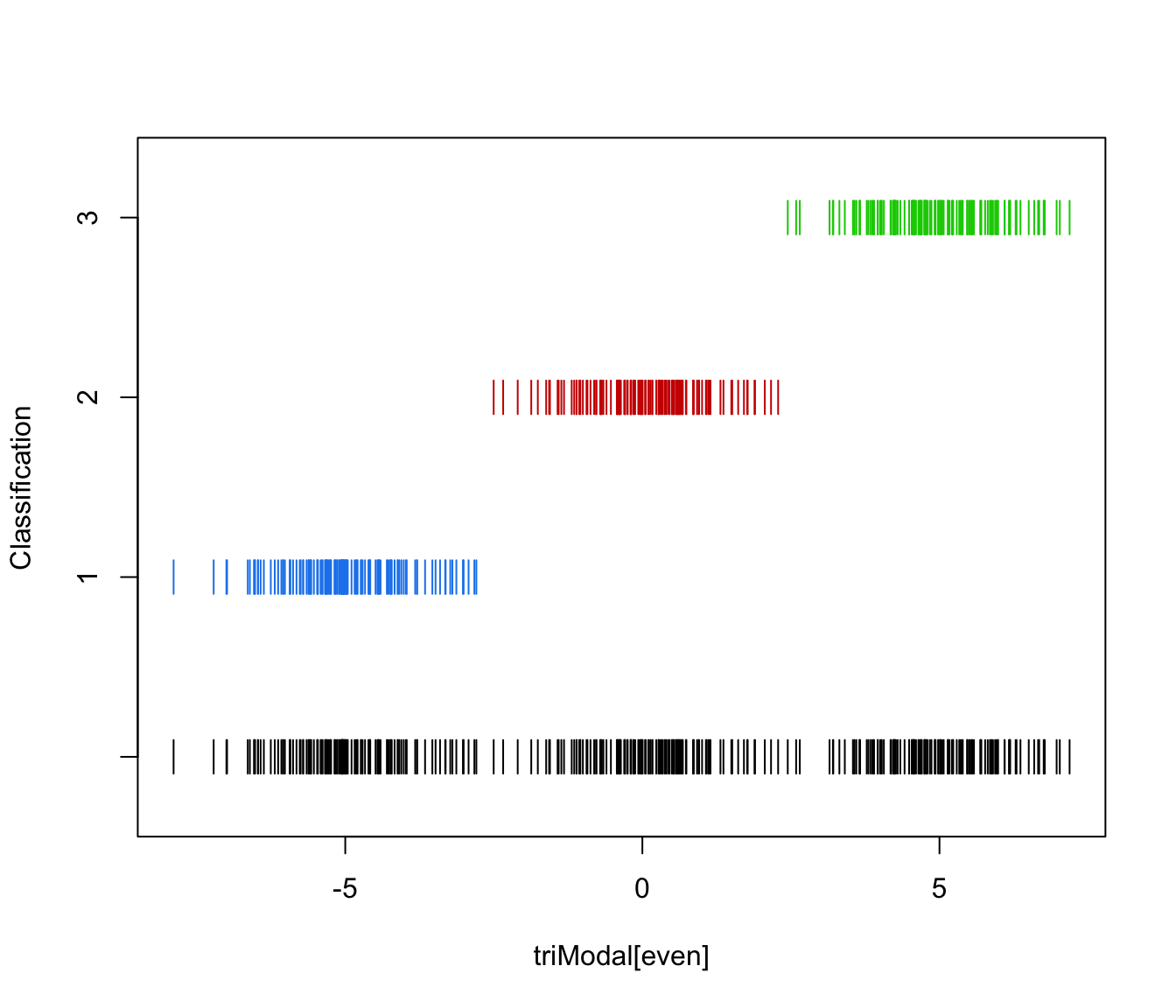 plot(triMclustDA, what = "train&test", newdata = triModal[even])
 plot(triMclustDA, what = "error")
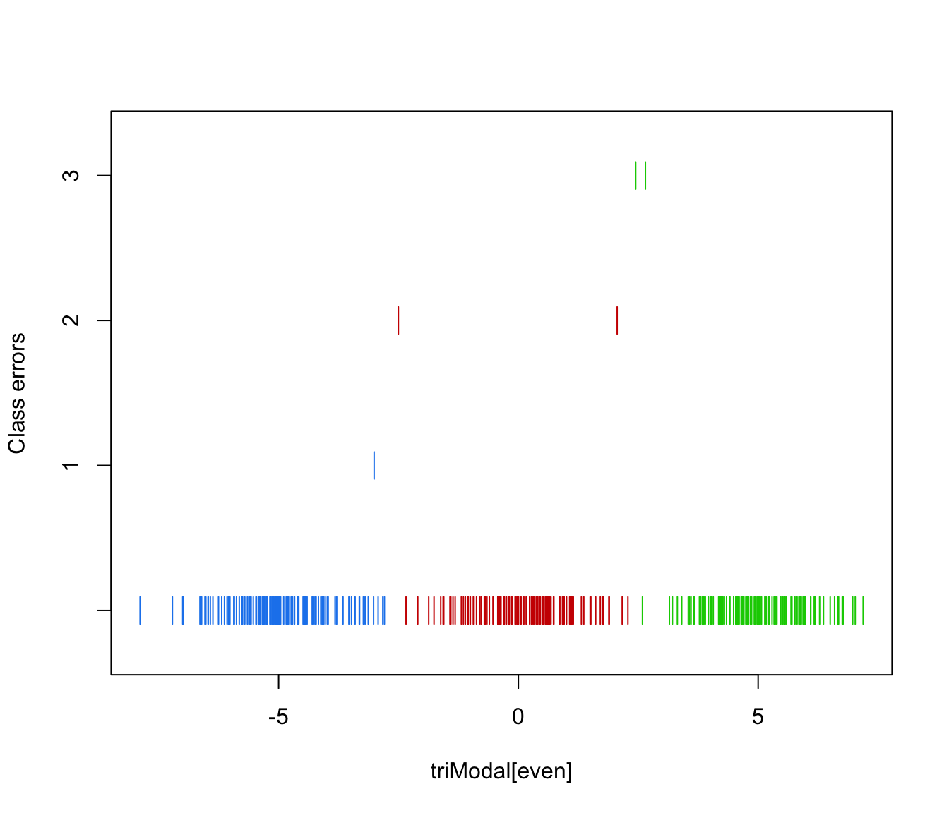
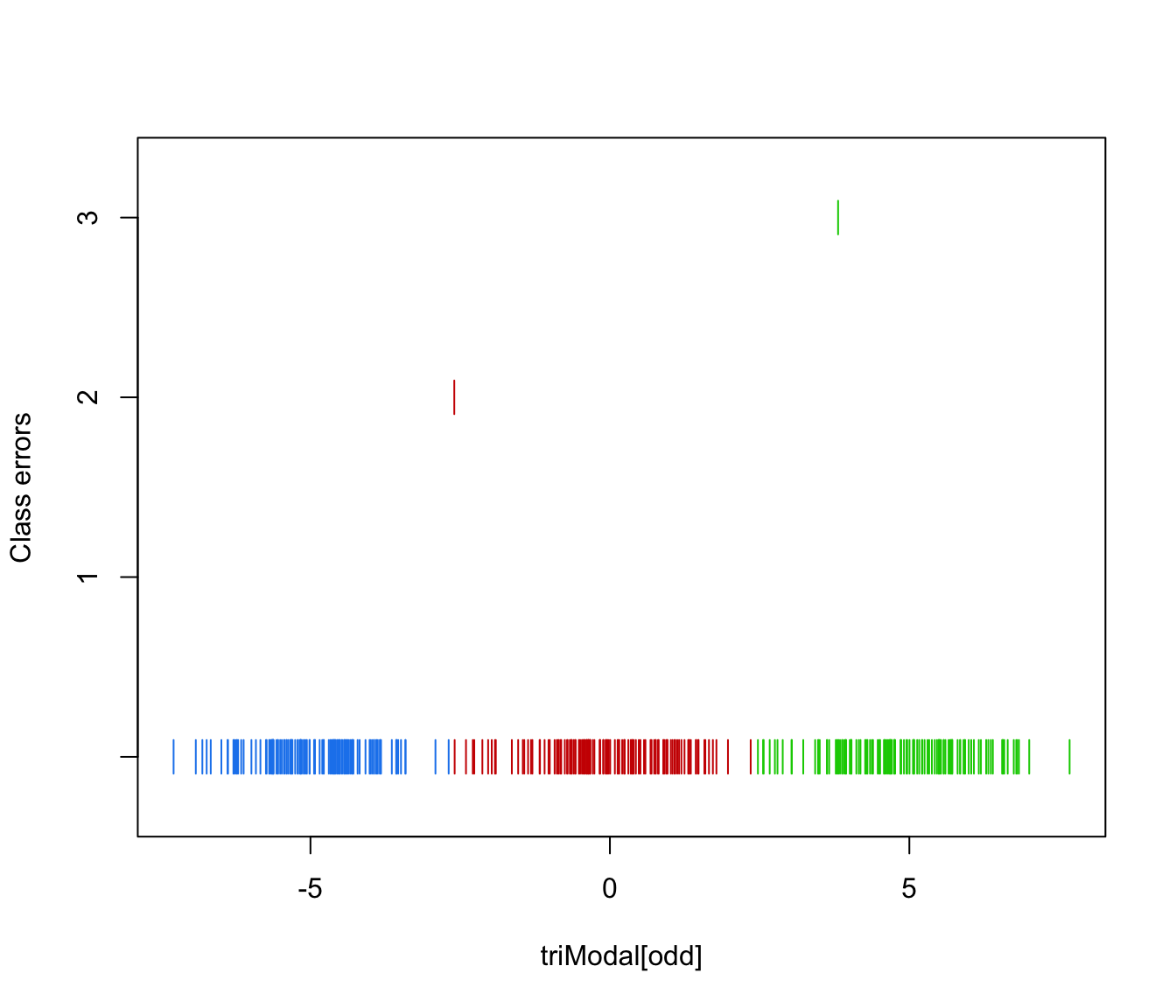 plot(triMclustDA, what = "error", newdata = triModal[even], newclass = triClass[even])
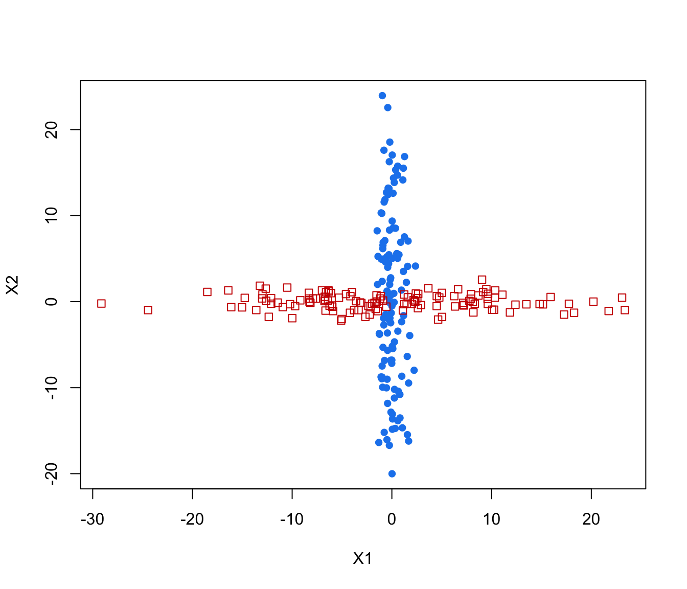
 # simulated 2D cross data
data(cross)
odd <- seq(from = 1, to = nrow(cross), by = 2)
even <- odd + 1
crossMclustDA <- MclustDA(cross[odd,-1], cross[odd,1])
summary(crossMclustDA, parameters = TRUE)
#> ------------------------------------------------
#> Gaussian finite mixture model for classification
#> ------------------------------------------------
#>
#> MclustDA
#> ------------------------------------------------
#> log-likelihood n df BIC
#> -1381.404 250 10 -2818.022
#>
#> Classes n % Model G
#> 1 125 50 XXX 1
#> 2 125 50 XXI 1
#>
#> Parameter estimates
#> ------------------------------------------------
#> Class prior probabilities:
#> 1 2
#> 0.5 0.5
#>
#> Class = 1
#> ---------
#>
#> Mixing probabilities: 1
#>
#> Means:
#> [,1]
#> X1 0.03982835
#> X2 -0.55982893
#>
#> Variances:
#> [,,1]
#> X1 X2
#> X1 1.030302 1.81975
#> X2 1.819750 72.90428
#>
#> Class = 2
#> ---------
#>
#> Mixing probabilities: 1
#>
#> Means:
#> [,1]
#> X1 0.2877120
#> X2 -0.1231171
#>
#> Variances:
#> [,,1]
#> X1 X2
#> X1 87.3583 0.0000000
#> X2 0.0000 0.8995777
#>
#> Training confusion matrix
#> ------------------------------------------------
#> Predicted
#> Classes 1 2
#> 1 112 13
#> 2 13 112
#>
#> Classification error = 0.1040
#> Brier score = 0.0563
summary(crossMclustDA, newdata = cross[even,-1], newclass = cross[even,1])
#> ------------------------------------------------
#> Gaussian finite mixture model for classification
#> ------------------------------------------------
#>
#> MclustDA
#> ------------------------------------------------
#> log-likelihood n df BIC
#> -1381.404 250 10 -2818.022
#>
#> Classes n % Model G
#> 1 125 50 XXX 1
#> 2 125 50 XXI 1
#>
#> Training confusion matrix
#> ------------------------------------------------
#> Predicted
#> Classes 1 2
#> 1 112 13
#> 2 13 112
#>
#> Classification error = 0.1040
#> Brier score = 0.0563
#>
#> Test confusion matrix
#> ------------------------------------------------
#> Predicted
#> Classes 1 2
#> 1 118 7
#> 2 5 120
#>
#> Classification error = 0.0480
#> Brier score = 0.0298
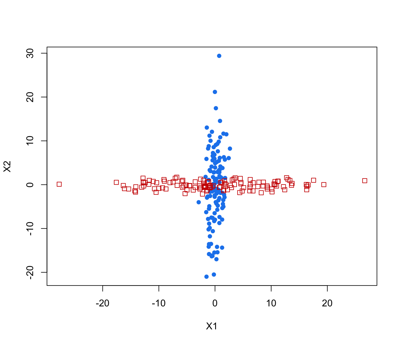
plot(crossMclustDA, what = "scatterplot")
# simulated 2D cross data
data(cross)
odd <- seq(from = 1, to = nrow(cross), by = 2)
even <- odd + 1
crossMclustDA <- MclustDA(cross[odd,-1], cross[odd,1])
summary(crossMclustDA, parameters = TRUE)
#> ------------------------------------------------
#> Gaussian finite mixture model for classification
#> ------------------------------------------------
#>
#> MclustDA
#> ------------------------------------------------
#> log-likelihood n df BIC
#> -1381.404 250 10 -2818.022
#>
#> Classes n % Model G
#> 1 125 50 XXX 1
#> 2 125 50 XXI 1
#>
#> Parameter estimates
#> ------------------------------------------------
#> Class prior probabilities:
#> 1 2
#> 0.5 0.5
#>
#> Class = 1
#> ---------
#>
#> Mixing probabilities: 1
#>
#> Means:
#> [,1]
#> X1 0.03982835
#> X2 -0.55982893
#>
#> Variances:
#> [,,1]
#> X1 X2
#> X1 1.030302 1.81975
#> X2 1.819750 72.90428
#>
#> Class = 2
#> ---------
#>
#> Mixing probabilities: 1
#>
#> Means:
#> [,1]
#> X1 0.2877120
#> X2 -0.1231171
#>
#> Variances:
#> [,,1]
#> X1 X2
#> X1 87.3583 0.0000000
#> X2 0.0000 0.8995777
#>
#> Training confusion matrix
#> ------------------------------------------------
#> Predicted
#> Classes 1 2
#> 1 112 13
#> 2 13 112
#>
#> Classification error = 0.1040
#> Brier score = 0.0563
summary(crossMclustDA, newdata = cross[even,-1], newclass = cross[even,1])
#> ------------------------------------------------
#> Gaussian finite mixture model for classification
#> ------------------------------------------------
#>
#> MclustDA
#> ------------------------------------------------
#> log-likelihood n df BIC
#> -1381.404 250 10 -2818.022
#>
#> Classes n % Model G
#> 1 125 50 XXX 1
#> 2 125 50 XXI 1
#>
#> Training confusion matrix
#> ------------------------------------------------
#> Predicted
#> Classes 1 2
#> 1 112 13
#> 2 13 112
#>
#> Classification error = 0.1040
#> Brier score = 0.0563
#>
#> Test confusion matrix
#> ------------------------------------------------
#> Predicted
#> Classes 1 2
#> 1 118 7
#> 2 5 120
#>
#> Classification error = 0.0480
#> Brier score = 0.0298
plot(crossMclustDA, what = "scatterplot")
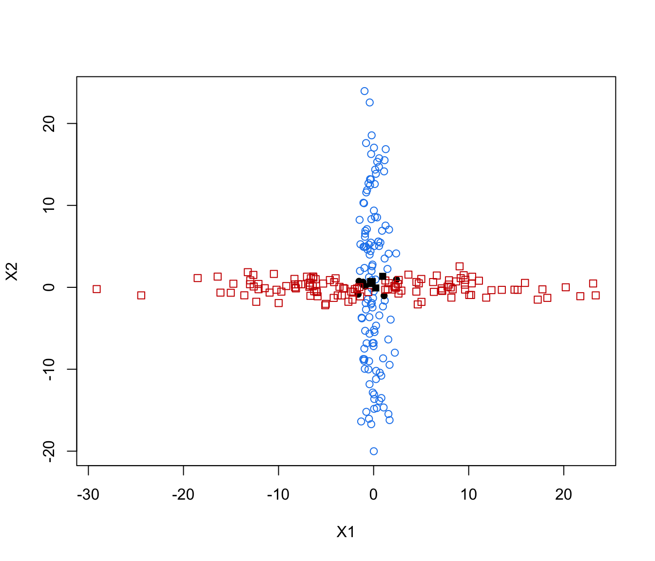
 plot(crossMclustDA, what = "classification")
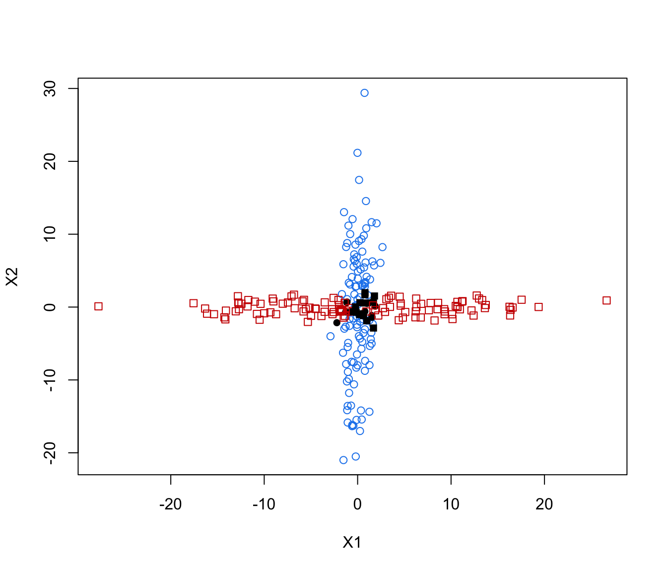
 plot(crossMclustDA, what = "classification", newdata = cross[even,-1])
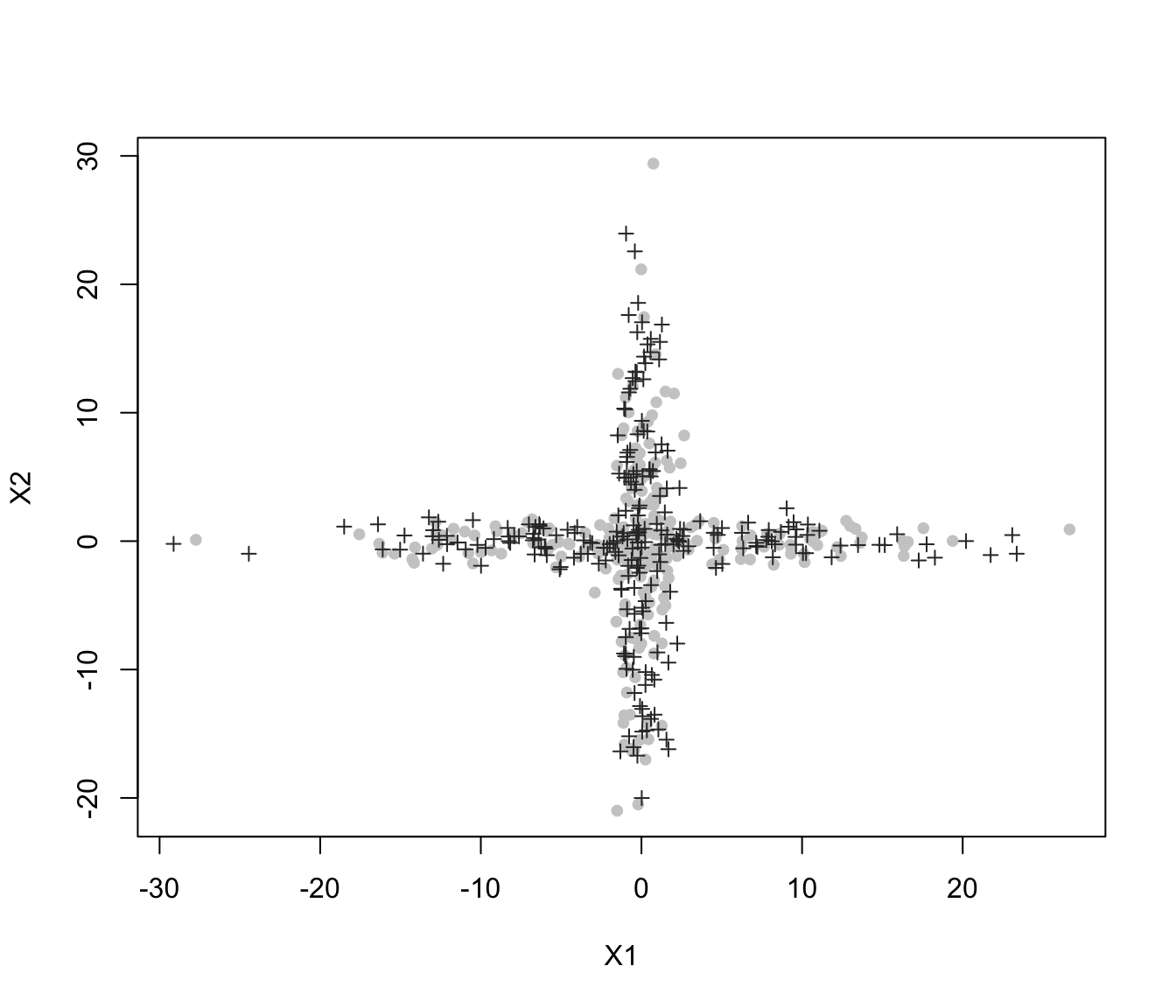
 plot(crossMclustDA, what = "train&test", newdata = cross[even,-1])
 plot(crossMclustDA, what = "error")
 plot(crossMclustDA, what = "error", newdata =cross[even,-1], newclass = cross[even,1])
 # }
# }