Plotting method for MclustDA discriminant analysis
plot.MclustDA.RdPlots for model-based mixture discriminant analysis results, such as scatterplot of training and test data, classification of train and test data, and errors.
Arguments
- x
An object of class
'MclustDA'resulting from a call toMclustDA.- what
A string specifying the type of graph requested. Available choices are:
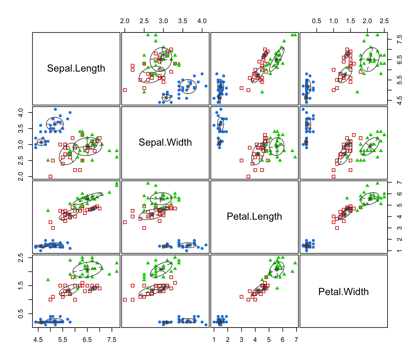
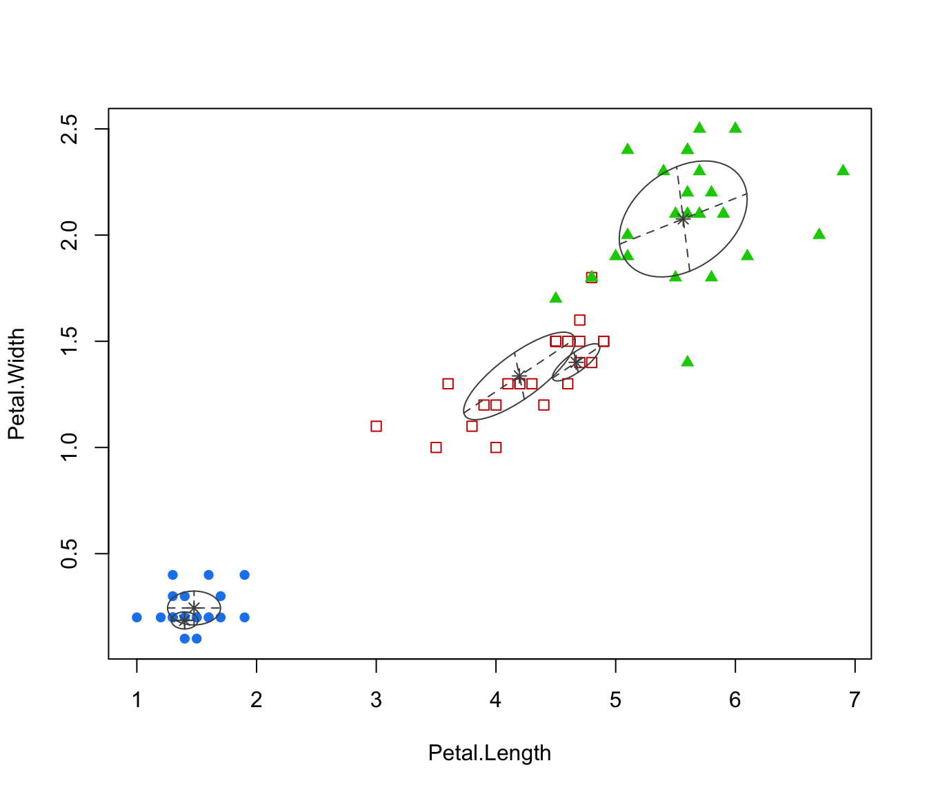
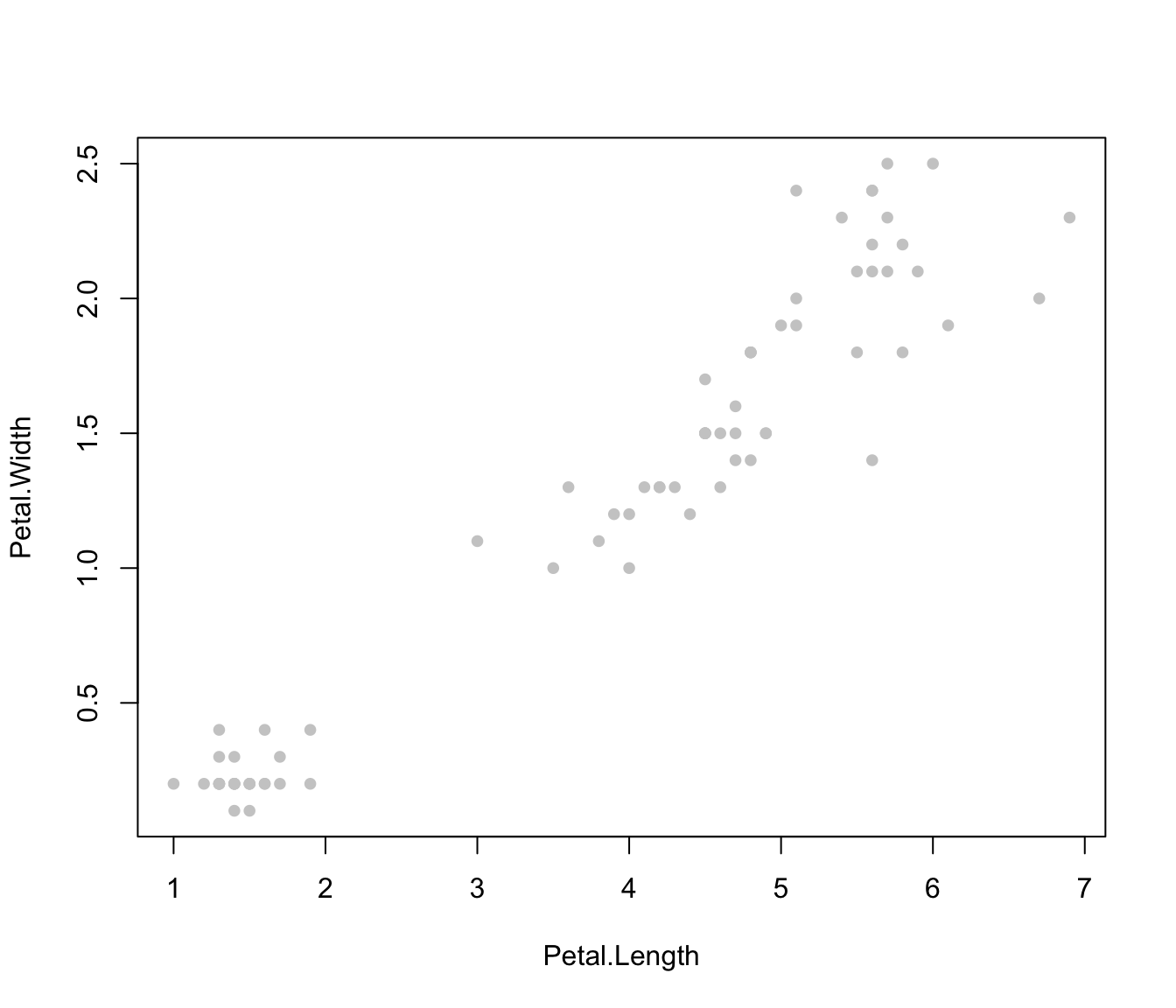
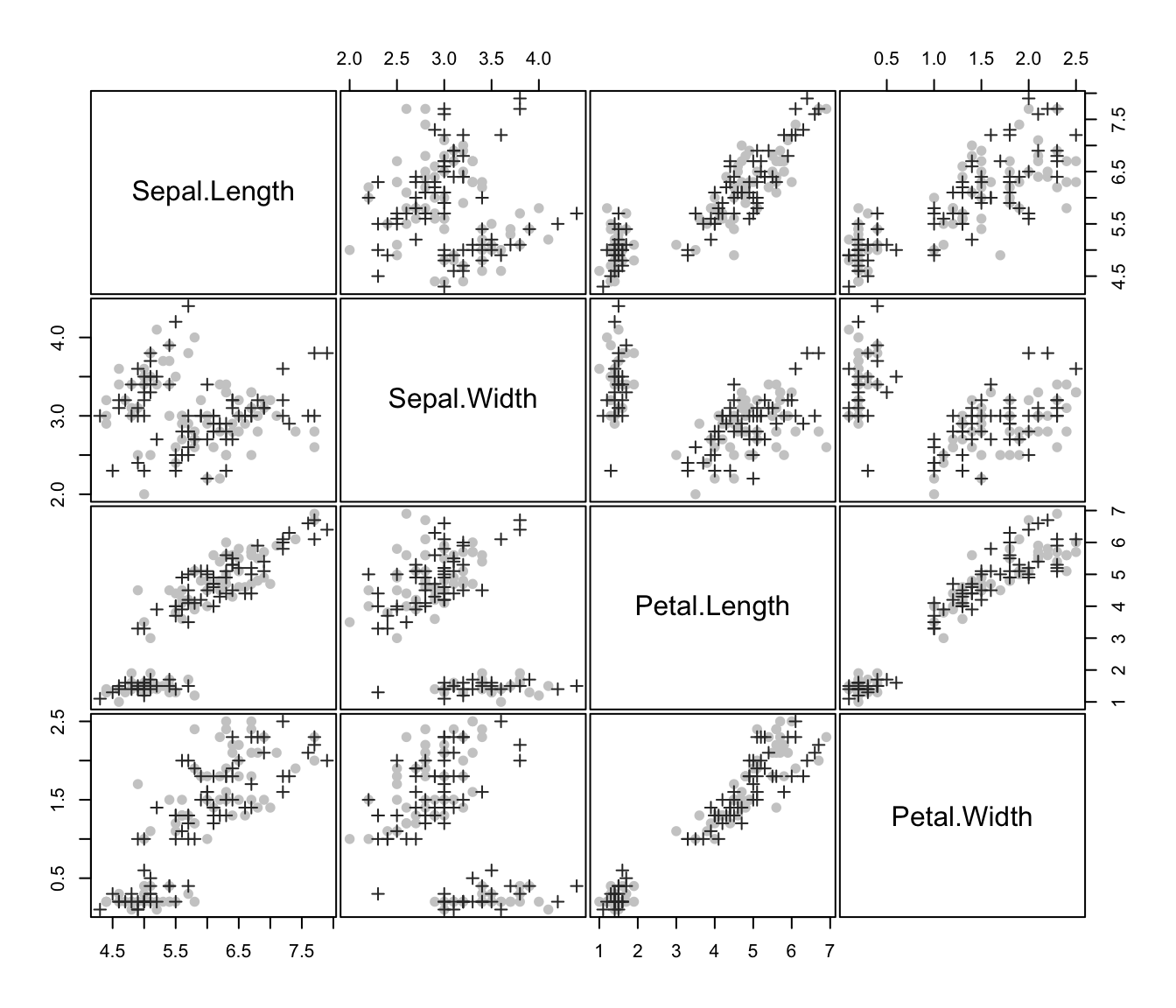
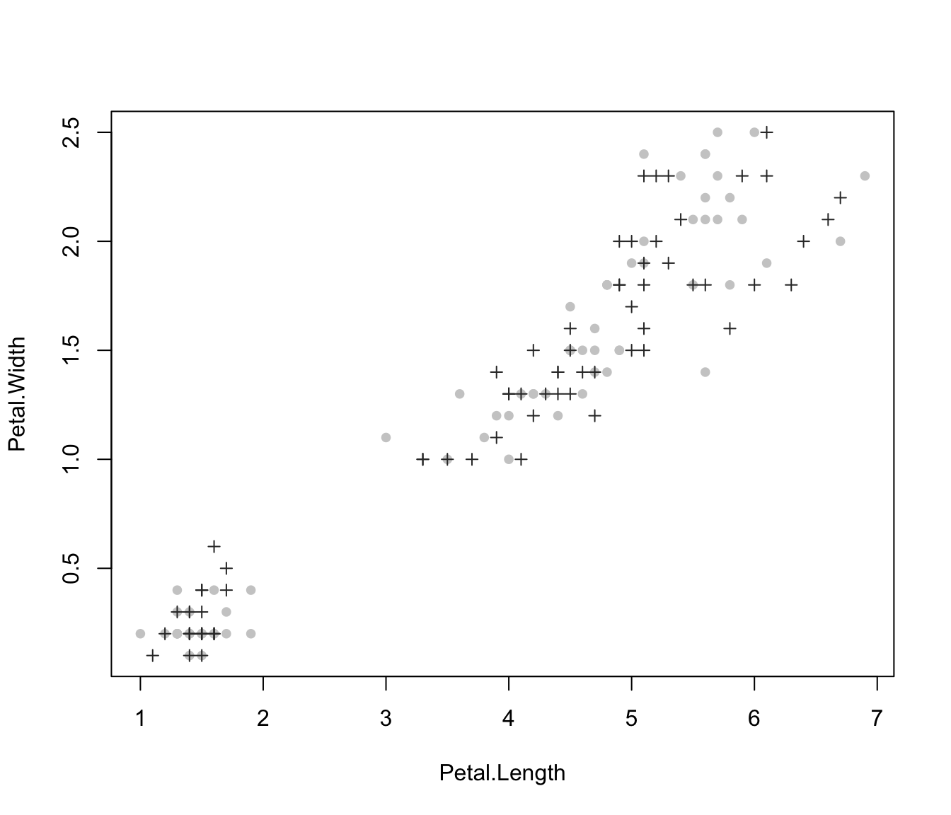
"scatterplot"=a plot of training data with points marked based on the known classification. Ellipses corresponding to covariances of mixture components are also drawn.
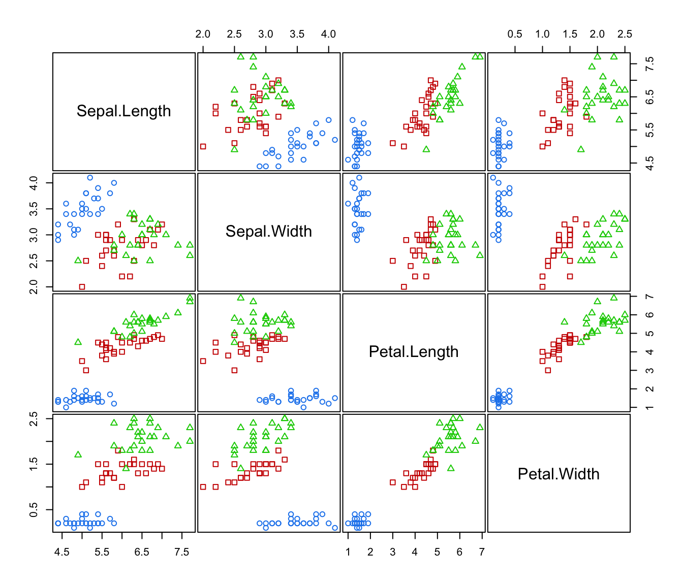
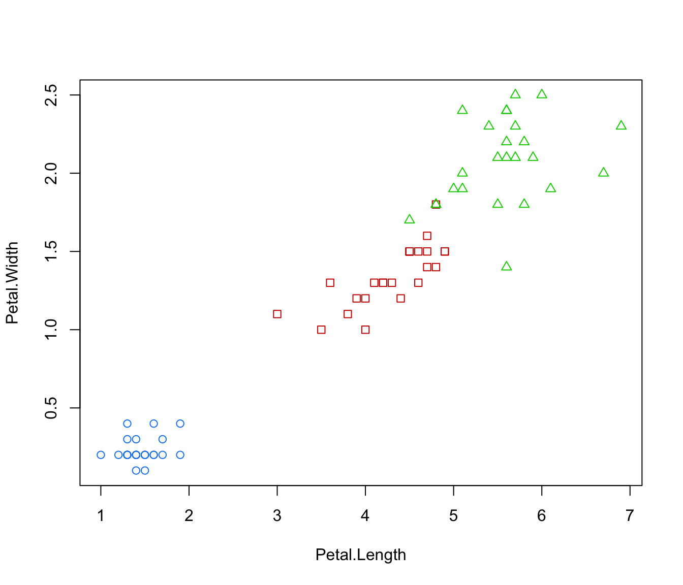
"classification"=a plot of data with points marked on based the predicted classification; if
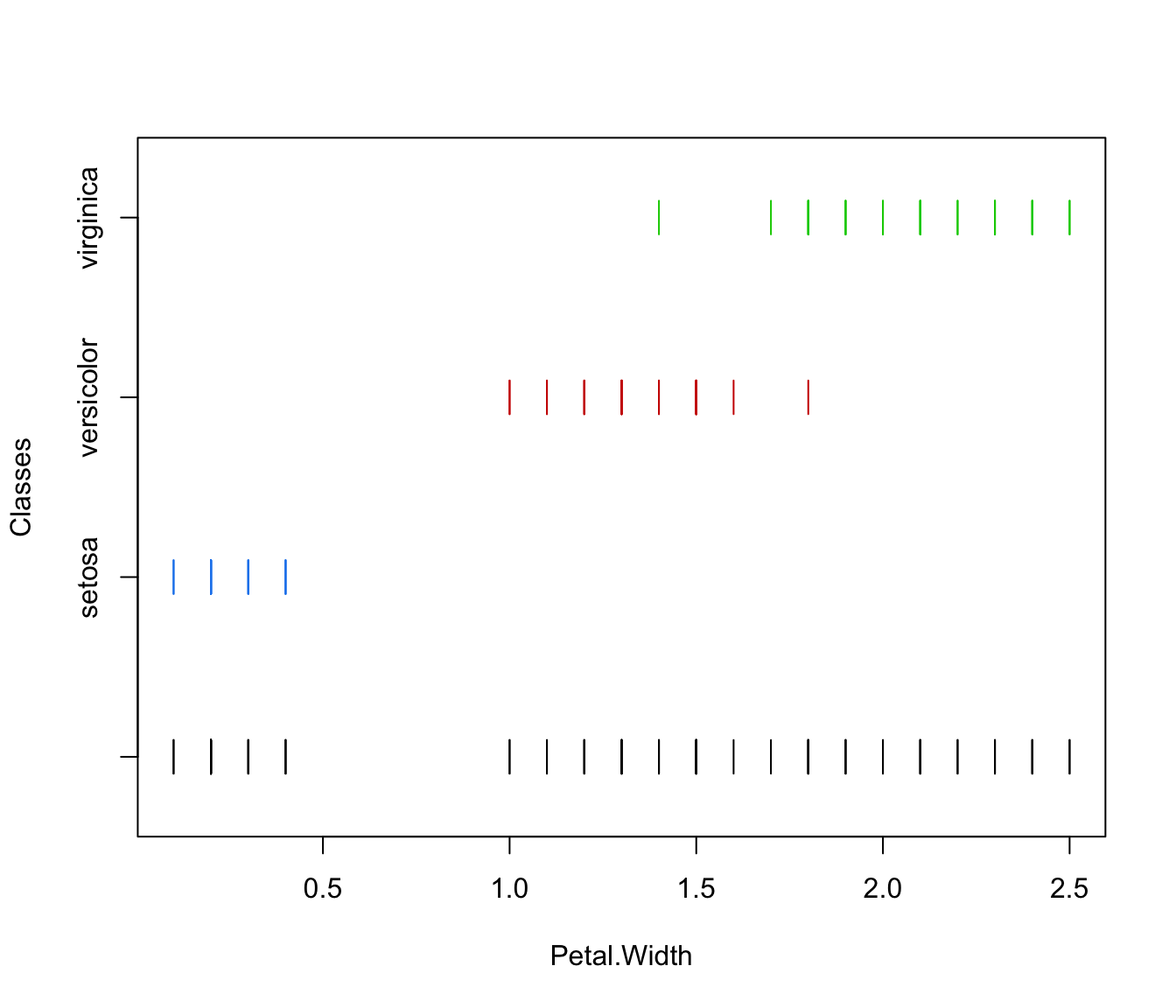
newdatais provided then the test set is shown otherwise the training set."train&test"=a plot of training and test data with points marked according to the type of set.
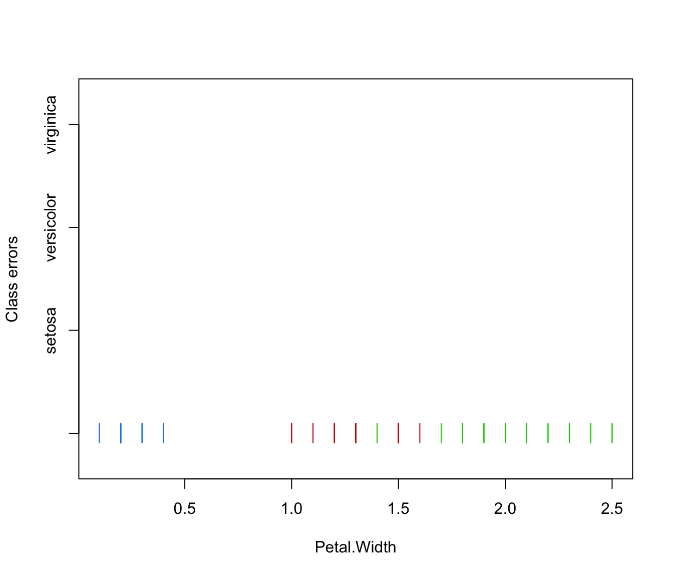
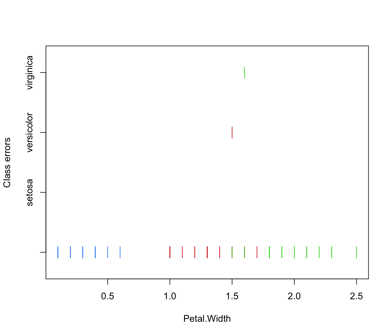
"error"=a plot of training set (or test set if
newdataandnewclassare provided) with misclassified points marked.
If not specified, in interactive sessions a menu of choices is proposed.
- newdata
A data frame or matrix for test data.
- newclass
A vector giving the class labels for the observations in the test data (if known).
- dimens
A vector of integers giving the dimensions of the desired coordinate projections for multivariate data. The default is to take all the the available dimensions for plotting.
- symbols
Either an integer or character vector assigning a plotting symbol to each unique class. Elements in
colorscorrespond to classes in order of appearance in the sequence of observations (the order used by the functionfactor). The default is given bymclust.options("classPlotSymbols").- colors
Either an integer or character vector assigning a color to each unique class in
classification. Elements incolorscorrespond to classes in order of appearance in the sequence of observations (the order used by the functionfactor). The default is given bymclust.options("classPlotColors").- main
A logical, a character string, or
NULL(default) for the main title. IfNULLorFALSEno title is added to a plot. IfTRUEa default title is added identifying the type of plot drawn. If a character string is provided, this is used for the title.- ...
further arguments passed to or from other methods.
Details
For more flexibility in plotting, use mclust1Dplot,
mclust2Dplot, surfacePlot, coordProj, or
randProj.
Examples
# \donttest{
odd <- seq(from = 1, to = nrow(iris), by = 2)
even <- odd + 1
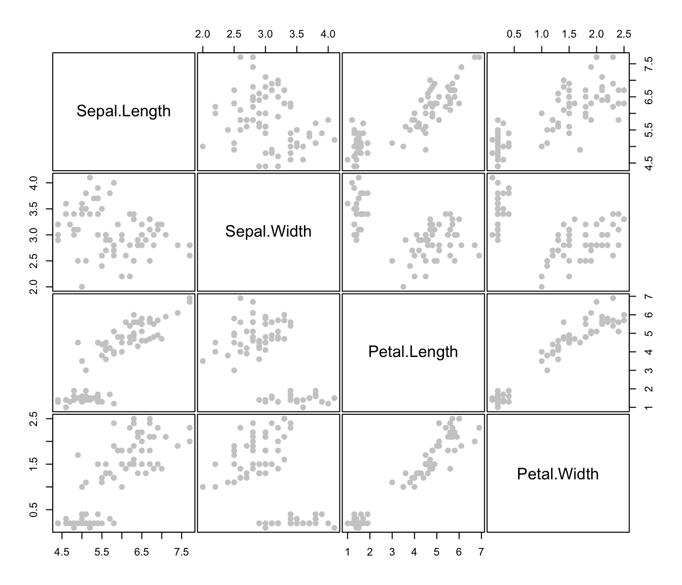
X.train <- iris[odd,-5]
Class.train <- iris[odd,5]
X.test <- iris[even,-5]
Class.test <- iris[even,5]
# common EEE covariance structure (which is essentially equivalent to linear discriminant analysis)
irisMclustDA <- MclustDA(X.train, Class.train, modelType = "EDDA", modelNames = "EEE")
summary(irisMclustDA, parameters = TRUE)
#> ------------------------------------------------
#> Gaussian finite mixture model for classification
#> ------------------------------------------------
#>
#> EDDA
#> ------------------------------------------------
#> log-likelihood n df BIC
#> -125.443 75 24 -354.5057
#>
#> Classes n % Model G
#> setosa 25 33.33 EEE 1
#> versicolor 25 33.33 EEE 1
#> virginica 25 33.33 EEE 1
#>
#> Parameter estimates
#> ------------------------------------------------
#> Class prior probabilities:
#> setosa versicolor virginica
#> 0.3333333 0.3333333 0.3333333
#>
#> Class = setosa
#> --------------
#>
#> Means:
#> [,1]
#> Sepal.Length 5.024
#> Sepal.Width 3.480
#> Petal.Length 1.456
#> Petal.Width 0.228
#>
#> Variances:
#> [,,1]
#> Sepal.Length Sepal.Width Petal.Length Petal.Width
#> Sepal.Length 0.26418133 0.06244800 0.15935467 0.03141333
#> Sepal.Width 0.06244800 0.09630933 0.03326933 0.03222400
#> Petal.Length 0.15935467 0.03326933 0.18236800 0.04091733
#> Petal.Width 0.03141333 0.03222400 0.04091733 0.03891200
#>
#> Class = versicolor
#> ------------------
#>
#> Means:
#> [,1]
#> Sepal.Length 5.992
#> Sepal.Width 2.776
#> Petal.Length 4.308
#> Petal.Width 1.352
#>
#> Variances:
#> [,,1]
#> Sepal.Length Sepal.Width Petal.Length Petal.Width
#> Sepal.Length 0.26418133 0.06244800 0.15935467 0.03141333
#> Sepal.Width 0.06244800 0.09630933 0.03326933 0.03222400
#> Petal.Length 0.15935467 0.03326933 0.18236800 0.04091733
#> Petal.Width 0.03141333 0.03222400 0.04091733 0.03891200
#>
#> Class = virginica
#> -----------------
#>
#> Means:
#> [,1]
#> Sepal.Length 6.504
#> Sepal.Width 2.936
#> Petal.Length 5.564
#> Petal.Width 2.076
#>
#> Variances:
#> [,,1]
#> Sepal.Length Sepal.Width Petal.Length Petal.Width
#> Sepal.Length 0.26418133 0.06244800 0.15935467 0.03141333
#> Sepal.Width 0.06244800 0.09630933 0.03326933 0.03222400
#> Petal.Length 0.15935467 0.03326933 0.18236800 0.04091733
#> Petal.Width 0.03141333 0.03222400 0.04091733 0.03891200
#>
#> Training confusion matrix
#> ------------------------------------------------
#> Predicted
#> Classes setosa versicolor virginica
#> setosa 25 0 0
#> versicolor 0 24 1
#> virginica 0 1 24
#>
#> Classification error = 0.0267
#> Brier score = 0.0097
summary(irisMclustDA, newdata = X.test, newclass = Class.test)
#> ------------------------------------------------
#> Gaussian finite mixture model for classification
#> ------------------------------------------------
#>
#> EDDA
#> ------------------------------------------------
#> log-likelihood n df BIC
#> -125.443 75 24 -354.5057
#>
#> Classes n % Model G
#> setosa 25 33.33 EEE 1
#> versicolor 25 33.33 EEE 1
#> virginica 25 33.33 EEE 1
#>
#> Training confusion matrix
#> ------------------------------------------------
#> Predicted
#> Classes setosa versicolor virginica
#> setosa 25 0 0
#> versicolor 0 24 1
#> virginica 0 1 24
#>
#> Classification error = 0.0267
#> Brier score = 0.0097
#>
#> Test confusion matrix
#> ------------------------------------------------
#> Predicted
#> Classes setosa versicolor virginica
#> setosa 25 0 0
#> versicolor 0 24 1
#> virginica 0 2 23
#>
#> Classification error = 0.0400
#> Brier score = 0.0243
# common covariance structure selected by BIC
irisMclustDA <- MclustDA(X.train, Class.train, modelType = "EDDA")
summary(irisMclustDA, parameters = TRUE)
#> ------------------------------------------------
#> Gaussian finite mixture model for classification
#> ------------------------------------------------
#>
#> EDDA
#> ------------------------------------------------
#> log-likelihood n df BIC
#> -87.93758 75 38 -339.9397
#>
#> Classes n % Model G
#> setosa 25 33.33 VEV 1
#> versicolor 25 33.33 VEV 1
#> virginica 25 33.33 VEV 1
#>
#> Parameter estimates
#> ------------------------------------------------
#> Class prior probabilities:
#> setosa versicolor virginica
#> 0.3333333 0.3333333 0.3333333
#>
#> Class = setosa
#> --------------
#>
#> Means:
#> [,1]
#> Sepal.Length 5.024
#> Sepal.Width 3.480
#> Petal.Length 1.456
#> Petal.Width 0.228
#>
#> Variances:
#> [,,1]
#> Sepal.Length Sepal.Width Petal.Length Petal.Width
#> Sepal.Length 0.154450439 0.097646496 0.017347101 0.005327878
#> Sepal.Width 0.097646496 0.105230813 0.004066916 0.005599939
#> Petal.Length 0.017347101 0.004066916 0.041742267 0.003476241
#> Petal.Width 0.005327878 0.005599939 0.003476241 0.006454832
#>
#> Class = versicolor
#> ------------------
#>
#> Means:
#> [,1]
#> Sepal.Length 5.992
#> Sepal.Width 2.776
#> Petal.Length 4.308
#> Petal.Width 1.352
#>
#> Variances:
#> [,,1]
#> Sepal.Length Sepal.Width Petal.Length Petal.Width
#> Sepal.Length 0.26653496 0.06976610 0.17015657 0.04336127
#> Sepal.Width 0.06976610 0.09861066 0.07509657 0.03823057
#> Petal.Length 0.17015657 0.07509657 0.19799871 0.06126251
#> Petal.Width 0.04336127 0.03823057 0.06126251 0.03627058
#>
#> Class = virginica
#> -----------------
#>
#> Means:
#> [,1]
#> Sepal.Length 6.504
#> Sepal.Width 2.936
#> Petal.Length 5.564
#> Petal.Width 2.076
#>
#> Variances:
#> [,,1]
#> Sepal.Length Sepal.Width Petal.Length Petal.Width
#> Sepal.Length 0.37570480 0.025364426 0.280227270 0.03871029
#> Sepal.Width 0.02536443 0.080872957 0.006413281 0.05009229
#> Petal.Length 0.28022727 0.006413281 0.309059434 0.05805268
#> Petal.Width 0.03871029 0.050092291 0.058052679 0.07540425
#>
#> Training confusion matrix
#> ------------------------------------------------
#> Predicted
#> Classes setosa versicolor virginica
#> setosa 25 0 0
#> versicolor 0 24 1
#> virginica 0 0 25
#>
#> Classification error = 0.0133
#> Brier score = 0.0054
summary(irisMclustDA, newdata = X.test, newclass = Class.test)
#> ------------------------------------------------
#> Gaussian finite mixture model for classification
#> ------------------------------------------------
#>
#> EDDA
#> ------------------------------------------------
#> log-likelihood n df BIC
#> -87.93758 75 38 -339.9397
#>
#> Classes n % Model G
#> setosa 25 33.33 VEV 1
#> versicolor 25 33.33 VEV 1
#> virginica 25 33.33 VEV 1
#>
#> Training confusion matrix
#> ------------------------------------------------
#> Predicted
#> Classes setosa versicolor virginica
#> setosa 25 0 0
#> versicolor 0 24 1
#> virginica 0 0 25
#>
#> Classification error = 0.0133
#> Brier score = 0.0054
#>
#> Test confusion matrix
#> ------------------------------------------------
#> Predicted
#> Classes setosa versicolor virginica
#> setosa 25 0 0
#> versicolor 0 24 1
#> virginica 0 2 23
#>
#> Classification error = 0.0400
#> Brier score = 0.0297
# general covariance structure selected by BIC
irisMclustDA <- MclustDA(X.train, Class.train)
summary(irisMclustDA, parameters = TRUE)
#> ------------------------------------------------
#> Gaussian finite mixture model for classification
#> ------------------------------------------------
#>
#> MclustDA
#> ------------------------------------------------
#> log-likelihood n df BIC
#> -71.74193 75 50 -359.3583
#>
#> Classes n % Model G
#> setosa 25 33.33 VEI 2
#> versicolor 25 33.33 VEE 2
#> virginica 25 33.33 XXX 1
#>
#> Parameter estimates
#> ------------------------------------------------
#> Class prior probabilities:
#> setosa versicolor virginica
#> 0.3333333 0.3333333 0.3333333
#>
#> Class = setosa
#> --------------
#>
#> Mixing probabilities: 0.7229143 0.2770857
#>
#> Means:
#> [,1] [,2]
#> Sepal.Length 5.1761949 4.6269248
#> Sepal.Width 3.6366552 3.0712877
#> Petal.Length 1.4777585 1.3992323
#> Petal.Width 0.2441875 0.1857668
#>
#> Variances:
#> [,,1]
#> Sepal.Length Sepal.Width Petal.Length Petal.Width
#> Sepal.Length 0.120728 0.000000 0.00000000 0.000000000
#> Sepal.Width 0.000000 0.046461 0.00000000 0.000000000
#> Petal.Length 0.000000 0.000000 0.04892923 0.000000000
#> Petal.Width 0.000000 0.000000 0.00000000 0.006358681
#> [,,2]
#> Sepal.Length Sepal.Width Petal.Length Petal.Width
#> Sepal.Length 0.03044364 0.00000000 0.00000000 0.000000000
#> Sepal.Width 0.00000000 0.01171594 0.00000000 0.000000000
#> Petal.Length 0.00000000 0.00000000 0.01233835 0.000000000
#> Petal.Width 0.00000000 0.00000000 0.00000000 0.001603451
#>
#> Class = versicolor
#> ------------------
#>
#> Mixing probabilities: 0.2364317 0.7635683
#>
#> Means:
#> [,1] [,2]
#> Sepal.Length 6.736465 5.761483
#> Sepal.Width 3.000982 2.706336
#> Petal.Length 4.669933 4.195931
#> Petal.Width 1.400893 1.336861
#>
#> Variances:
#> [,,1]
#> Sepal.Length Sepal.Width Petal.Length Petal.Width
#> Sepal.Length 0.030012918 0.008262520 0.02533959 0.008673053
#> Sepal.Width 0.008262520 0.020600060 0.01200205 0.008400168
#> Petal.Length 0.025339590 0.012002053 0.03924151 0.013788157
#> Petal.Width 0.008673053 0.008400168 0.01378816 0.007666627
#> [,,2]
#> Sepal.Length Sepal.Width Petal.Length Petal.Width
#> Sepal.Length 0.16630011 0.04578222 0.14040543 0.04805696
#> Sepal.Width 0.04578222 0.11414392 0.06650279 0.04654492
#> Petal.Length 0.14040543 0.06650279 0.21743528 0.07639950
#> Petal.Width 0.04805696 0.04654492 0.07639950 0.04248041
#>
#> Class = virginica
#> -----------------
#>
#> Mixing probabilities: 1
#>
#> Means:
#> [,1]
#> Sepal.Length 6.504
#> Sepal.Width 2.936
#> Petal.Length 5.564
#> Petal.Width 2.076
#>
#> Variances:
#> [,,1]
#> Sepal.Length Sepal.Width Petal.Length Petal.Width
#> Sepal.Length 0.349184 0.019056 0.272144 0.040896
#> Sepal.Width 0.019056 0.079104 0.011296 0.048064
#> Petal.Length 0.272144 0.011296 0.285504 0.049536
#> Petal.Width 0.040896 0.048064 0.049536 0.074624
#>
#> Training confusion matrix
#> ------------------------------------------------
#> Predicted
#> Classes setosa versicolor virginica
#> setosa 25 0 0
#> versicolor 0 25 0
#> virginica 0 0 25
#>
#> Classification error = 0.0000
#> Brier score = 0.0041
summary(irisMclustDA, newdata = X.test, newclass = Class.test)
#> ------------------------------------------------
#> Gaussian finite mixture model for classification
#> ------------------------------------------------
#>
#> MclustDA
#> ------------------------------------------------
#> log-likelihood n df BIC
#> -71.74193 75 50 -359.3583
#>
#> Classes n % Model G
#> setosa 25 33.33 VEI 2
#> versicolor 25 33.33 VEE 2
#> virginica 25 33.33 XXX 1
#>
#> Training confusion matrix
#> ------------------------------------------------
#> Predicted
#> Classes setosa versicolor virginica
#> setosa 25 0 0
#> versicolor 0 25 0
#> virginica 0 0 25
#>
#> Classification error = 0.0000
#> Brier score = 0.0041
#>
#> Test confusion matrix
#> ------------------------------------------------
#> Predicted
#> Classes setosa versicolor virginica
#> setosa 25 0 0
#> versicolor 0 24 1
#> virginica 0 1 24
#>
#> Classification error = 0.0267
#> Brier score = 0.0159
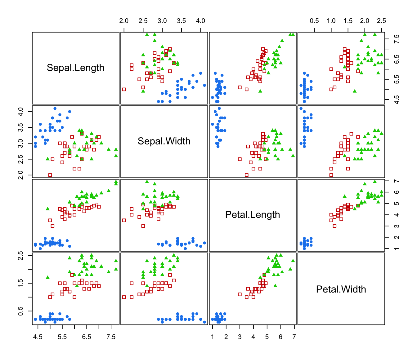
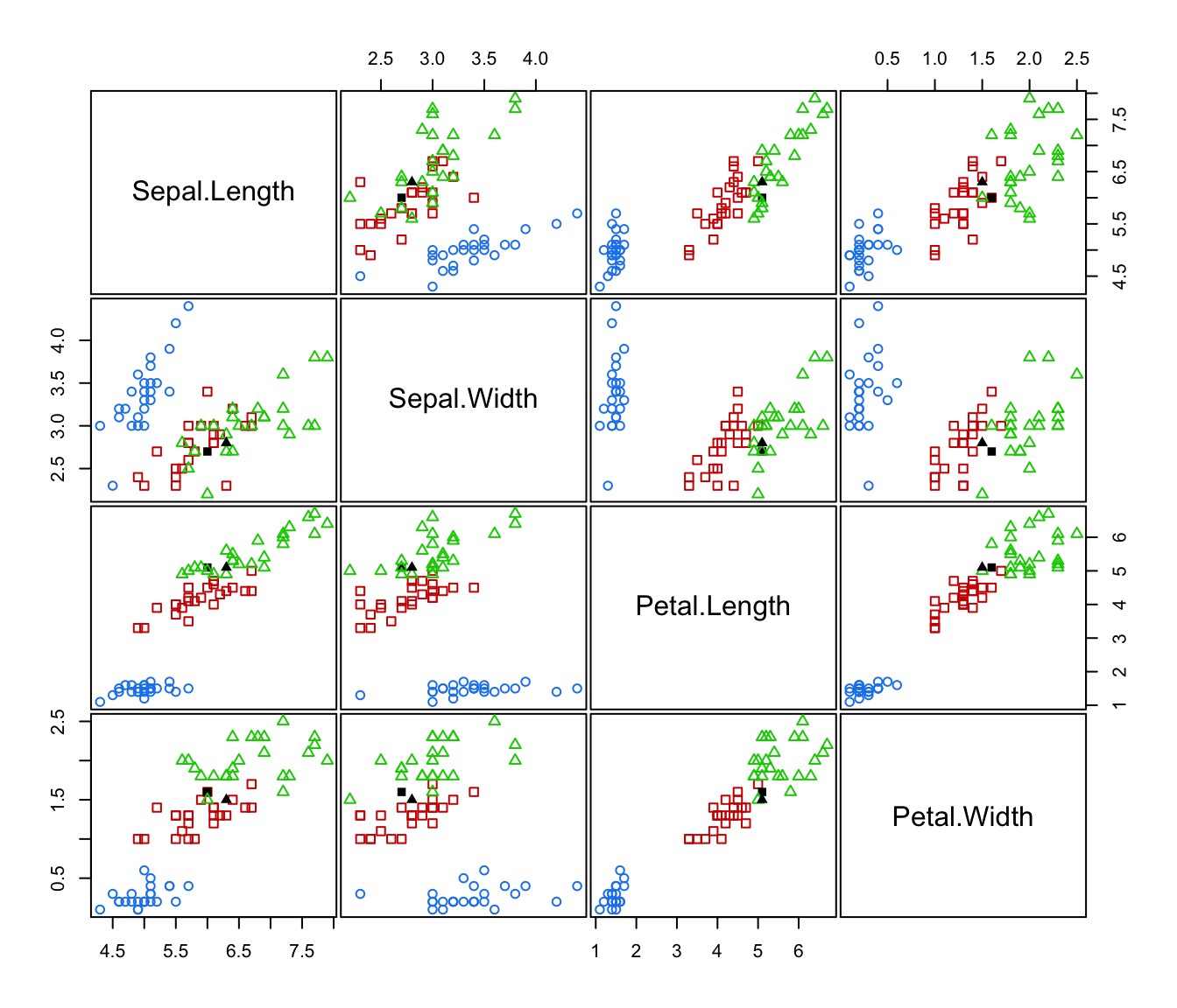
plot(irisMclustDA)

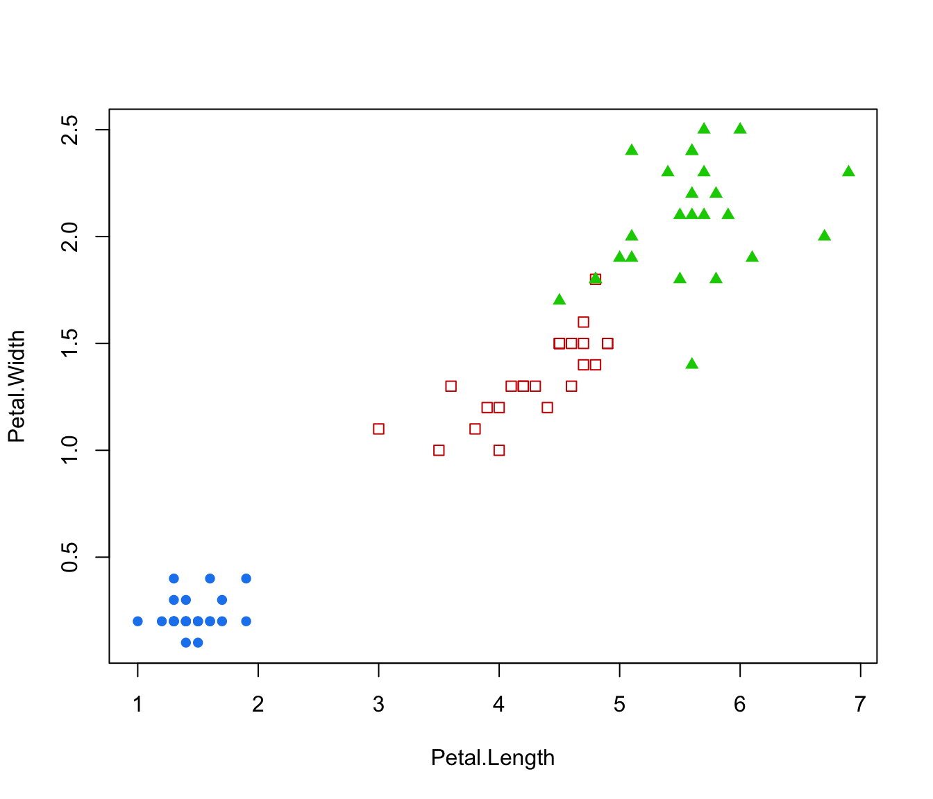
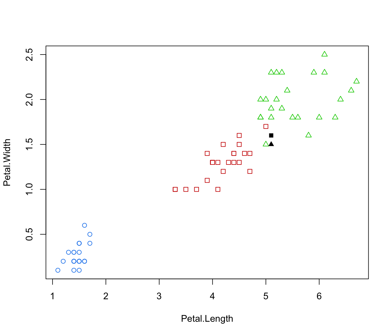
 plot(irisMclustDA, dimens = 3:4)

 plot(irisMclustDA, dimens = 4)


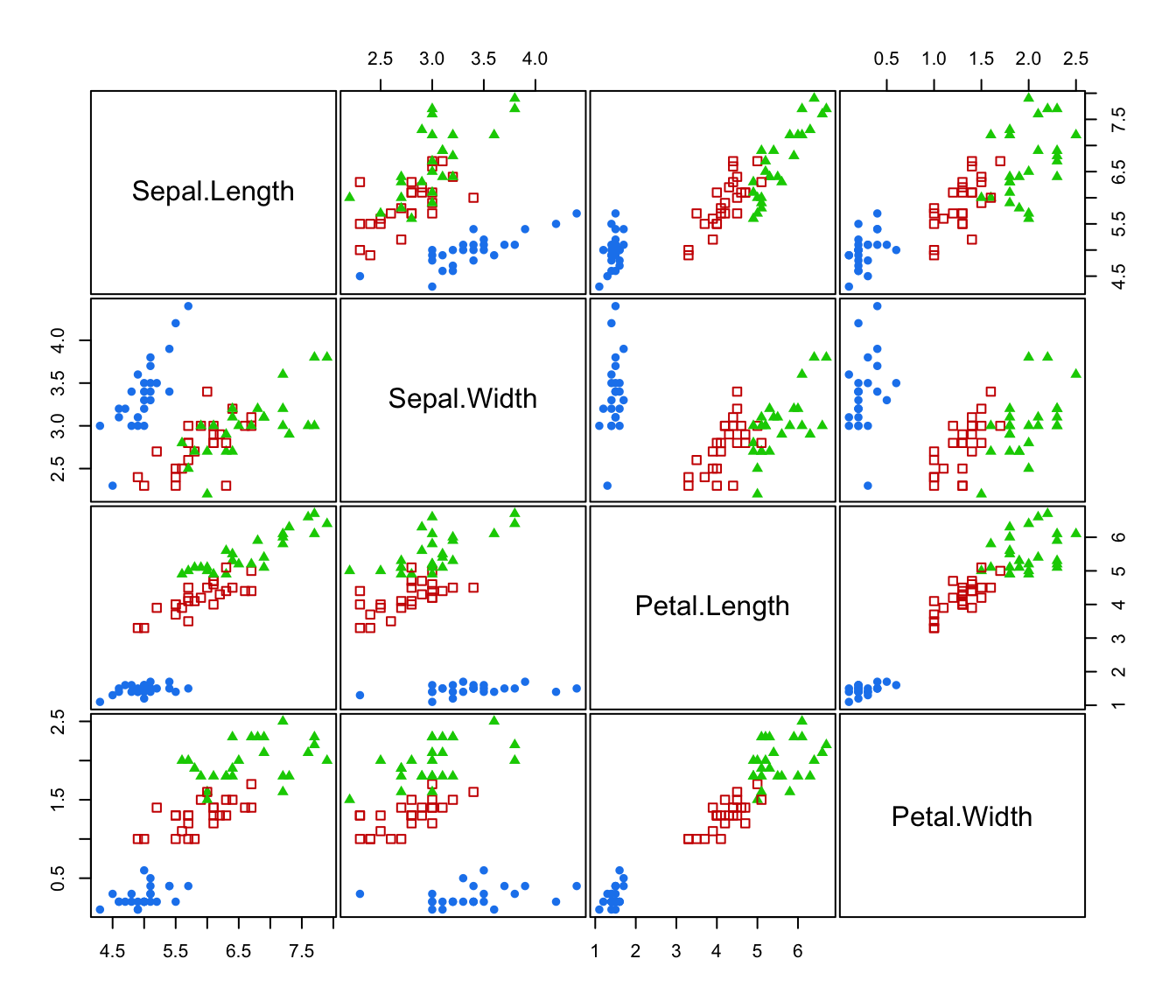
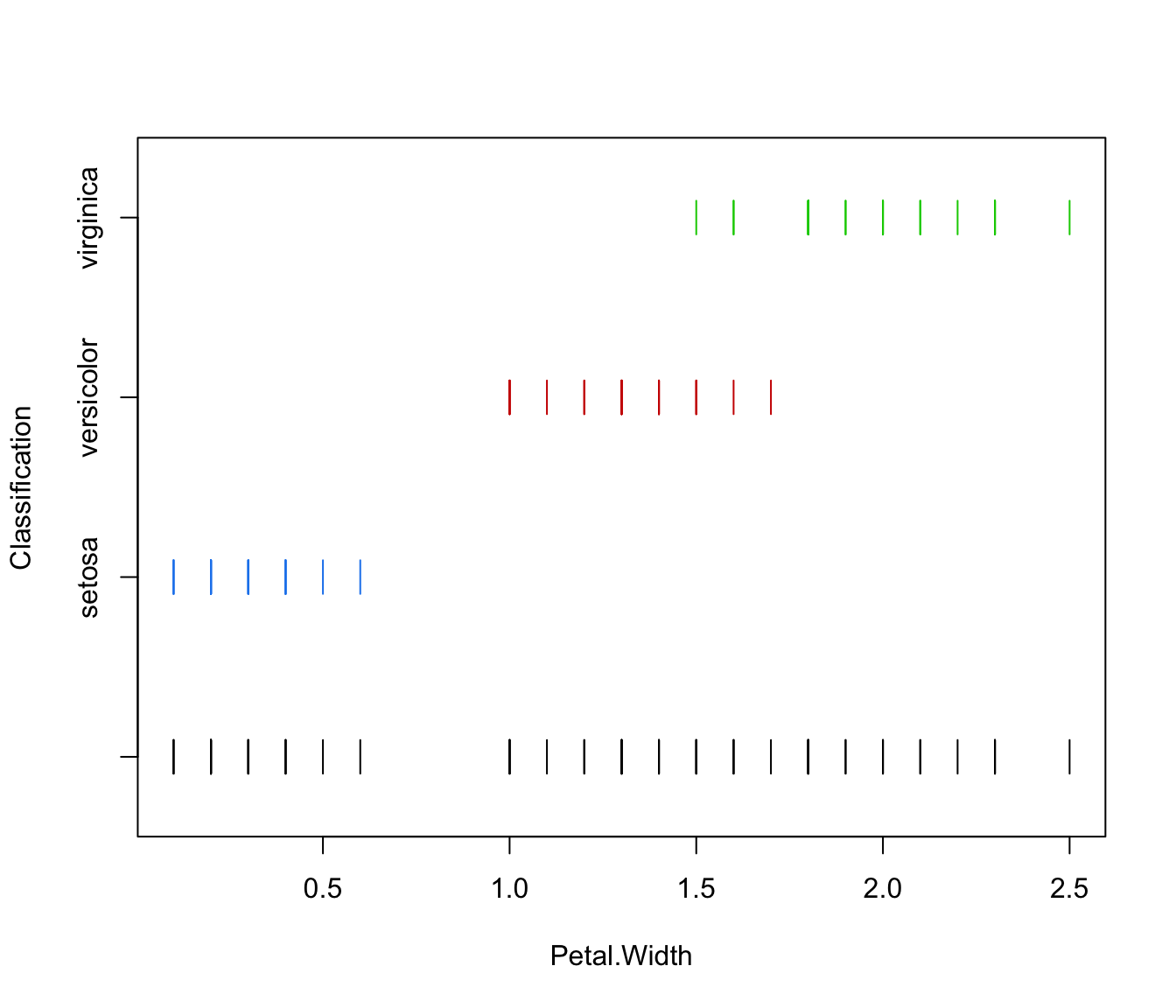
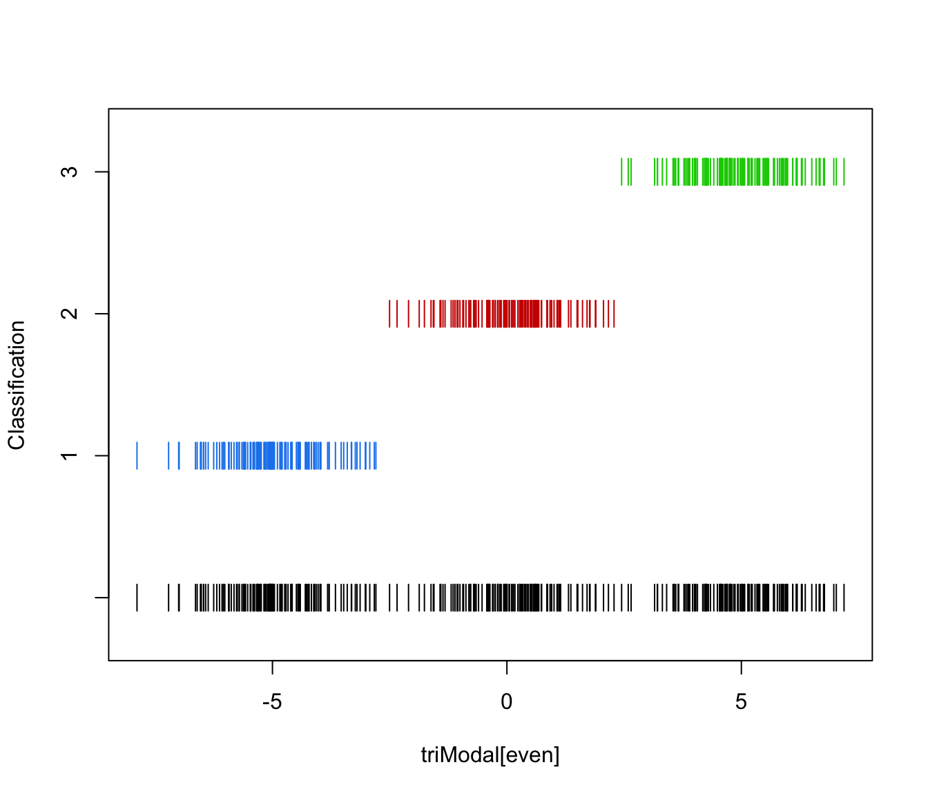
 plot(irisMclustDA, what = "classification")
 plot(irisMclustDA, what = "classification", newdata = X.test)
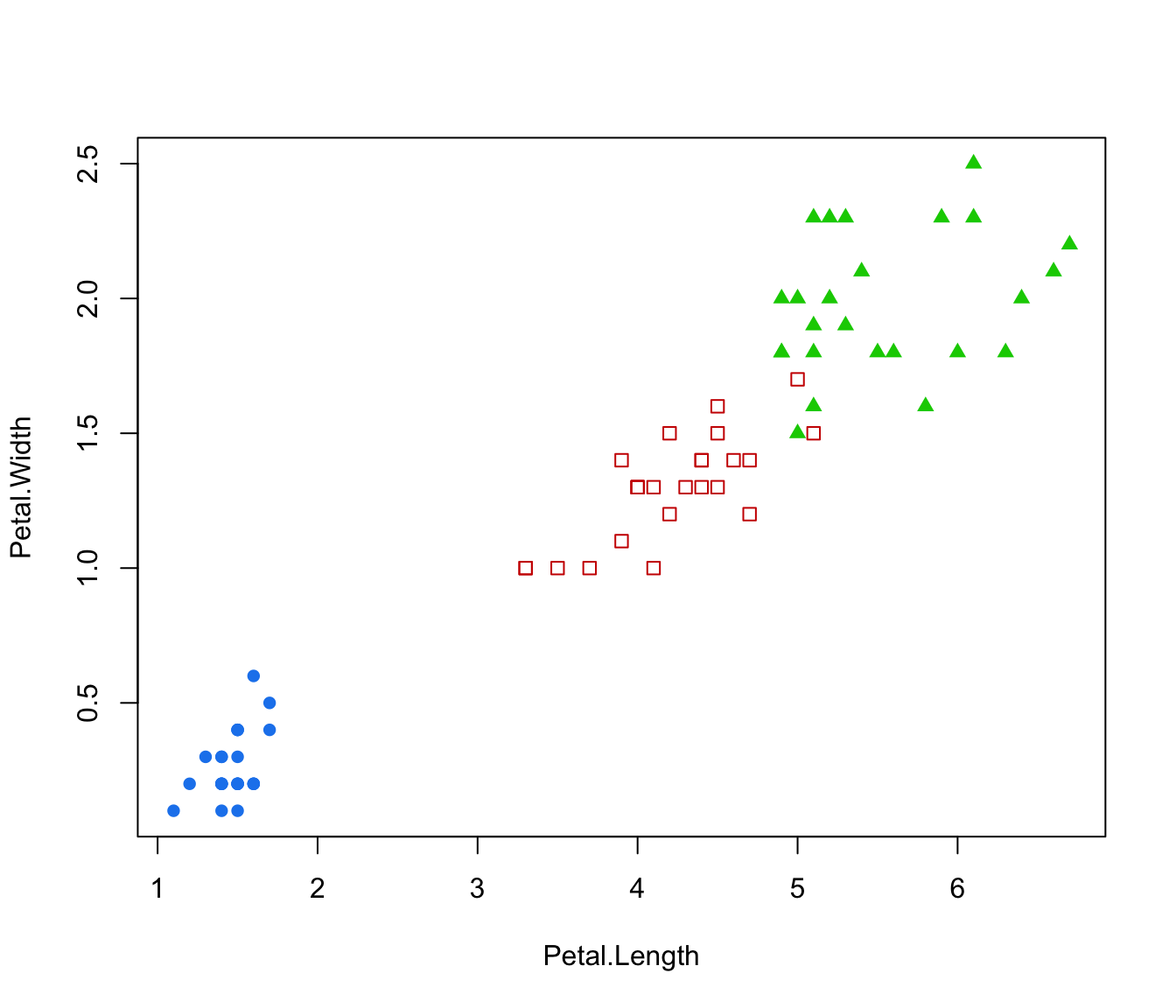
 plot(irisMclustDA, what = "classification", dimens = 3:4)
 plot(irisMclustDA, what = "classification", newdata = X.test, dimens = 3:4)
 plot(irisMclustDA, what = "classification", dimens = 4)
 plot(irisMclustDA, what = "classification", dimens = 4, newdata = X.test)
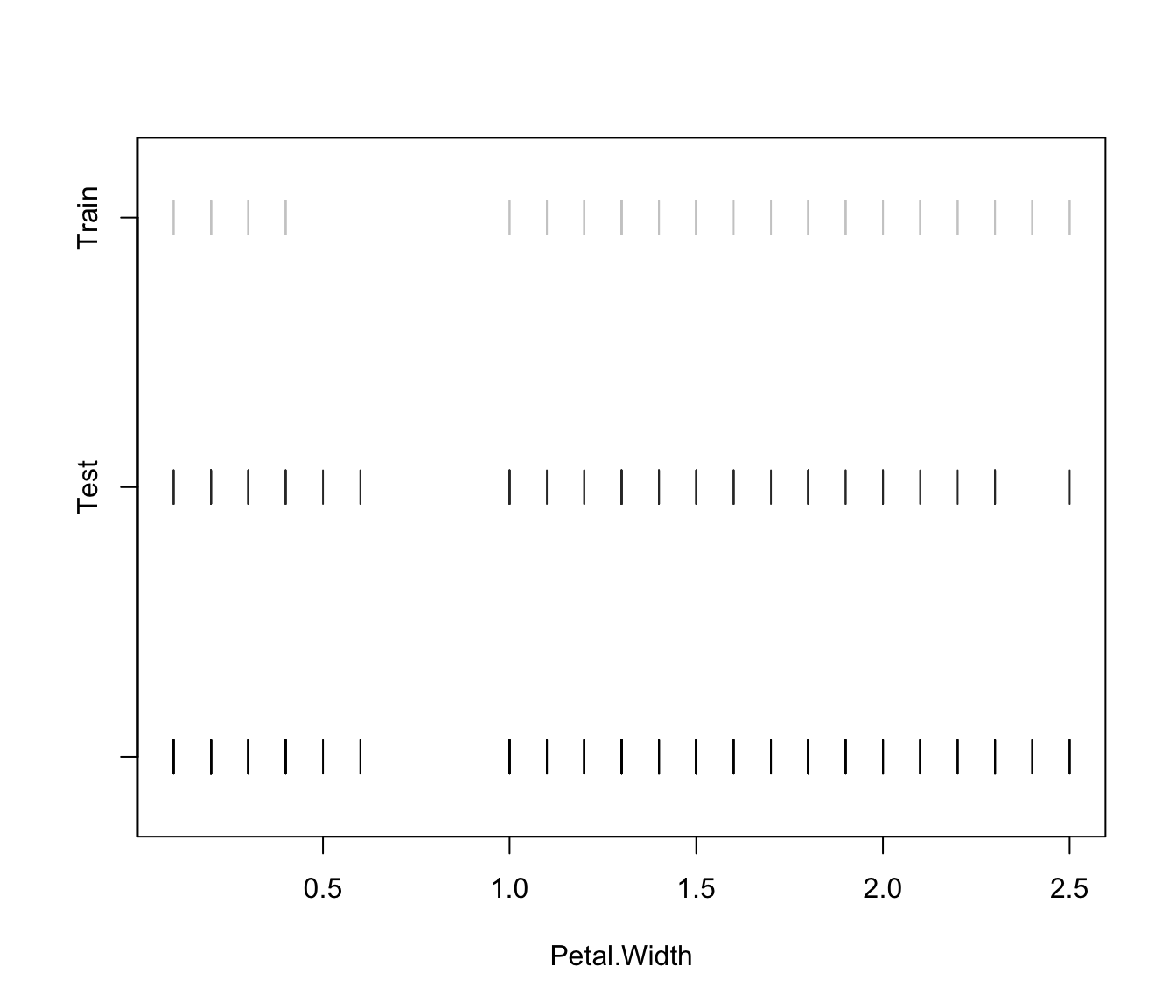
 plot(irisMclustDA, what = "train&test", newdata = X.test)
 plot(irisMclustDA, what = "train&test", newdata = X.test, dimens = 3:4)
 plot(irisMclustDA, what = "train&test", newdata = X.test, dimens = 4)
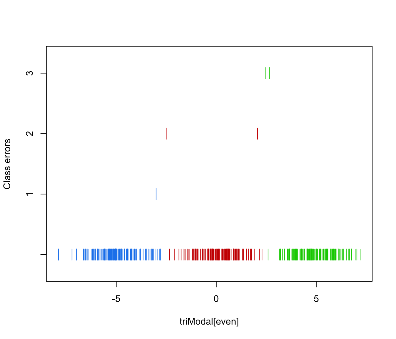
 plot(irisMclustDA, what = "error")
 plot(irisMclustDA, what = "error", dimens = 3:4)
 plot(irisMclustDA, what = "error", dimens = 4)
 plot(irisMclustDA, what = "error", newdata = X.test, newclass = Class.test)
 plot(irisMclustDA, what = "error", newdata = X.test, newclass = Class.test, dimens = 3:4)
 plot(irisMclustDA, what = "error", newdata = X.test, newclass = Class.test, dimens = 4)
 # simulated 1D data
n <- 250
set.seed(1)
triModal <- c(rnorm(n,-5), rnorm(n,0), rnorm(n,5))
triClass <- c(rep(1,n), rep(2,n), rep(3,n))
odd <- seq(from = 1, to = length(triModal), by = 2)
even <- odd + 1
triMclustDA <- MclustDA(triModal[odd], triClass[odd])
summary(triMclustDA, parameters = TRUE)
#> ------------------------------------------------
#> Gaussian finite mixture model for classification
#> ------------------------------------------------
#>
#> MclustDA
#> ------------------------------------------------
#> log-likelihood n df BIC
#> -942.4306 375 8 -1932.277
#>
#> Classes n % Model G
#> 1 125 33.33 X 1
#> 2 125 33.33 X 1
#> 3 125 33.33 X 1
#>
#> Parameter estimates
#> ------------------------------------------------
#> Class prior probabilities:
#> 1 2 3
#> 0.3333333 0.3333333 0.3333333
#>
#> Class = 1
#> ---------
#>
#> Mixing probabilities: 1
#>
#> Means:
#> [1] -4.951981
#>
#> Variances:
#> [1] 0.8268339
#>
#> Class = 2
#> ---------
#>
#> Mixing probabilities: 1
#>
#> Means:
#> [1] -0.01814707
#>
#> Variances:
#> [1] 1.201987
#>
#> Class = 3
#> ---------
#>
#> Mixing probabilities: 1
#>
#> Means:
#> [1] 4.875429
#>
#> Variances:
#> [1] 1.200321
#>
#> Training confusion matrix
#> ------------------------------------------------
#> Predicted
#> Classes 1 2 3
#> 1 124 1 0
#> 2 0 124 1
#> 3 0 0 125
#>
#> Classification error = 0.0053
#> Brier score = 0.0073
summary(triMclustDA, newdata = triModal[even], newclass = triClass[even])
#> ------------------------------------------------
#> Gaussian finite mixture model for classification
#> ------------------------------------------------
#>
#> MclustDA
#> ------------------------------------------------
#> log-likelihood n df BIC
#> -942.4306 375 8 -1932.277
#>
#> Classes n % Model G
#> 1 125 33.33 X 1
#> 2 125 33.33 X 1
#> 3 125 33.33 X 1
#>
#> Training confusion matrix
#> ------------------------------------------------
#> Predicted
#> Classes 1 2 3
#> 1 124 1 0
#> 2 0 124 1
#> 3 0 0 125
#>
#> Classification error = 0.0053
#> Brier score = 0.0073
#>
#> Test confusion matrix
#> ------------------------------------------------
#> Predicted
#> Classes 1 2 3
#> 1 124 1 0
#> 2 1 122 2
#> 3 0 1 124
#>
#> Classification error = 0.0133
#> Brier score = 0.0089
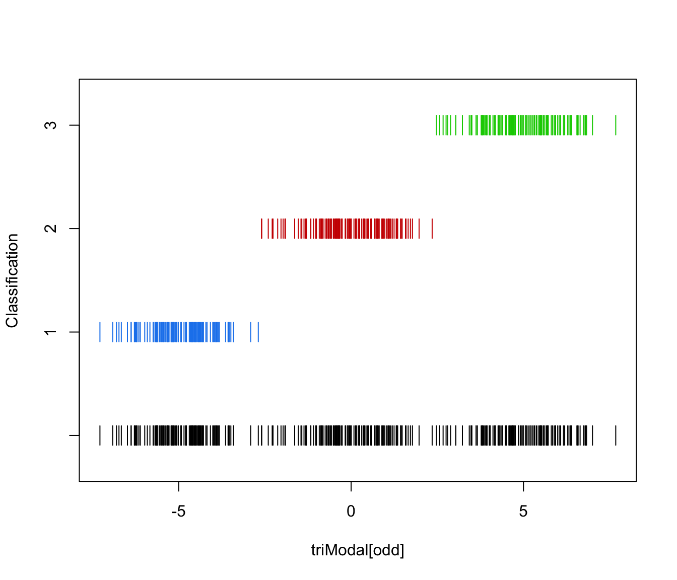
plot(triMclustDA)
# simulated 1D data
n <- 250
set.seed(1)
triModal <- c(rnorm(n,-5), rnorm(n,0), rnorm(n,5))
triClass <- c(rep(1,n), rep(2,n), rep(3,n))
odd <- seq(from = 1, to = length(triModal), by = 2)
even <- odd + 1
triMclustDA <- MclustDA(triModal[odd], triClass[odd])
summary(triMclustDA, parameters = TRUE)
#> ------------------------------------------------
#> Gaussian finite mixture model for classification
#> ------------------------------------------------
#>
#> MclustDA
#> ------------------------------------------------
#> log-likelihood n df BIC
#> -942.4306 375 8 -1932.277
#>
#> Classes n % Model G
#> 1 125 33.33 X 1
#> 2 125 33.33 X 1
#> 3 125 33.33 X 1
#>
#> Parameter estimates
#> ------------------------------------------------
#> Class prior probabilities:
#> 1 2 3
#> 0.3333333 0.3333333 0.3333333
#>
#> Class = 1
#> ---------
#>
#> Mixing probabilities: 1
#>
#> Means:
#> [1] -4.951981
#>
#> Variances:
#> [1] 0.8268339
#>
#> Class = 2
#> ---------
#>
#> Mixing probabilities: 1
#>
#> Means:
#> [1] -0.01814707
#>
#> Variances:
#> [1] 1.201987
#>
#> Class = 3
#> ---------
#>
#> Mixing probabilities: 1
#>
#> Means:
#> [1] 4.875429
#>
#> Variances:
#> [1] 1.200321
#>
#> Training confusion matrix
#> ------------------------------------------------
#> Predicted
#> Classes 1 2 3
#> 1 124 1 0
#> 2 0 124 1
#> 3 0 0 125
#>
#> Classification error = 0.0053
#> Brier score = 0.0073
summary(triMclustDA, newdata = triModal[even], newclass = triClass[even])
#> ------------------------------------------------
#> Gaussian finite mixture model for classification
#> ------------------------------------------------
#>
#> MclustDA
#> ------------------------------------------------
#> log-likelihood n df BIC
#> -942.4306 375 8 -1932.277
#>
#> Classes n % Model G
#> 1 125 33.33 X 1
#> 2 125 33.33 X 1
#> 3 125 33.33 X 1
#>
#> Training confusion matrix
#> ------------------------------------------------
#> Predicted
#> Classes 1 2 3
#> 1 124 1 0
#> 2 0 124 1
#> 3 0 0 125
#>
#> Classification error = 0.0053
#> Brier score = 0.0073
#>
#> Test confusion matrix
#> ------------------------------------------------
#> Predicted
#> Classes 1 2 3
#> 1 124 1 0
#> 2 1 122 2
#> 3 0 1 124
#>
#> Classification error = 0.0133
#> Brier score = 0.0089
plot(triMclustDA)


 plot(triMclustDA, what = "classification")
 plot(triMclustDA, what = "classification", newdata = triModal[even])
 plot(triMclustDA, what = "train&test", newdata = triModal[even])
 plot(triMclustDA, what = "error")
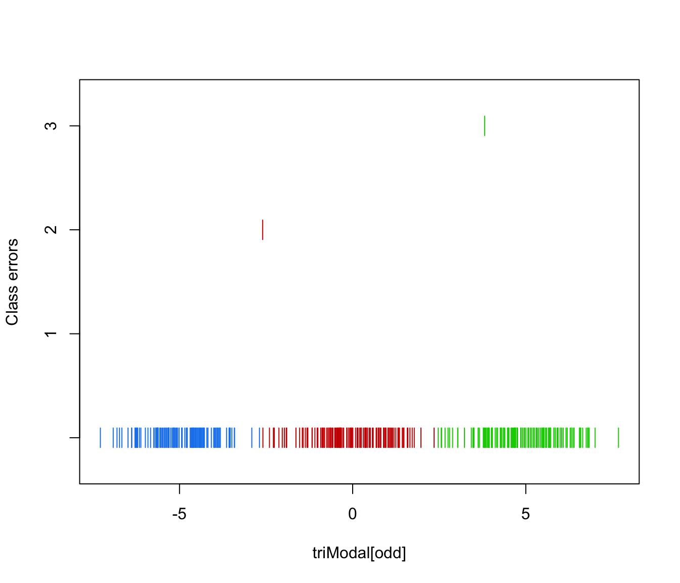 plot(triMclustDA, what = "error", newdata = triModal[even], newclass = triClass[even])
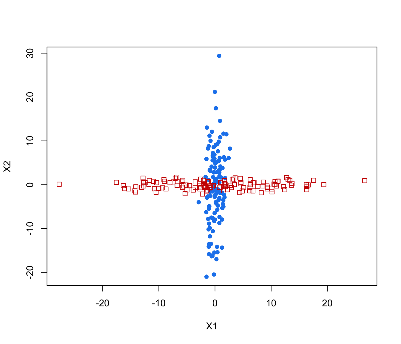
 # simulated 2D cross data
data(cross)
odd <- seq(from = 1, to = nrow(cross), by = 2)
even <- odd + 1
crossMclustDA <- MclustDA(cross[odd,-1], cross[odd,1])
summary(crossMclustDA, parameters = TRUE)
#> ------------------------------------------------
#> Gaussian finite mixture model for classification
#> ------------------------------------------------
#>
#> MclustDA
#> ------------------------------------------------
#> log-likelihood n df BIC
#> -1381.404 250 10 -2818.022
#>
#> Classes n % Model G
#> 1 125 50 XXX 1
#> 2 125 50 XXI 1
#>
#> Parameter estimates
#> ------------------------------------------------
#> Class prior probabilities:
#> 1 2
#> 0.5 0.5
#>
#> Class = 1
#> ---------
#>
#> Mixing probabilities: 1
#>
#> Means:
#> [,1]
#> X1 0.03982835
#> X2 -0.55982893
#>
#> Variances:
#> [,,1]
#> X1 X2
#> X1 1.030302 1.81975
#> X2 1.819750 72.90428
#>
#> Class = 2
#> ---------
#>
#> Mixing probabilities: 1
#>
#> Means:
#> [,1]
#> X1 0.2877120
#> X2 -0.1231171
#>
#> Variances:
#> [,,1]
#> X1 X2
#> X1 87.3583 0.0000000
#> X2 0.0000 0.8995777
#>
#> Training confusion matrix
#> ------------------------------------------------
#> Predicted
#> Classes 1 2
#> 1 112 13
#> 2 13 112
#>
#> Classification error = 0.1040
#> Brier score = 0.0563
summary(crossMclustDA, newdata = cross[even,-1], newclass = cross[even,1])
#> ------------------------------------------------
#> Gaussian finite mixture model for classification
#> ------------------------------------------------
#>
#> MclustDA
#> ------------------------------------------------
#> log-likelihood n df BIC
#> -1381.404 250 10 -2818.022
#>
#> Classes n % Model G
#> 1 125 50 XXX 1
#> 2 125 50 XXI 1
#>
#> Training confusion matrix
#> ------------------------------------------------
#> Predicted
#> Classes 1 2
#> 1 112 13
#> 2 13 112
#>
#> Classification error = 0.1040
#> Brier score = 0.0563
#>
#> Test confusion matrix
#> ------------------------------------------------
#> Predicted
#> Classes 1 2
#> 1 118 7
#> 2 5 120
#>
#> Classification error = 0.0480
#> Brier score = 0.0298
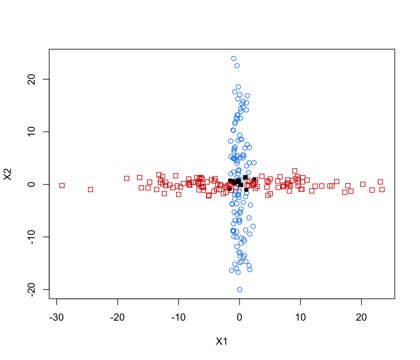
plot(crossMclustDA)
# simulated 2D cross data
data(cross)
odd <- seq(from = 1, to = nrow(cross), by = 2)
even <- odd + 1
crossMclustDA <- MclustDA(cross[odd,-1], cross[odd,1])
summary(crossMclustDA, parameters = TRUE)
#> ------------------------------------------------
#> Gaussian finite mixture model for classification
#> ------------------------------------------------
#>
#> MclustDA
#> ------------------------------------------------
#> log-likelihood n df BIC
#> -1381.404 250 10 -2818.022
#>
#> Classes n % Model G
#> 1 125 50 XXX 1
#> 2 125 50 XXI 1
#>
#> Parameter estimates
#> ------------------------------------------------
#> Class prior probabilities:
#> 1 2
#> 0.5 0.5
#>
#> Class = 1
#> ---------
#>
#> Mixing probabilities: 1
#>
#> Means:
#> [,1]
#> X1 0.03982835
#> X2 -0.55982893
#>
#> Variances:
#> [,,1]
#> X1 X2
#> X1 1.030302 1.81975
#> X2 1.819750 72.90428
#>
#> Class = 2
#> ---------
#>
#> Mixing probabilities: 1
#>
#> Means:
#> [,1]
#> X1 0.2877120
#> X2 -0.1231171
#>
#> Variances:
#> [,,1]
#> X1 X2
#> X1 87.3583 0.0000000
#> X2 0.0000 0.8995777
#>
#> Training confusion matrix
#> ------------------------------------------------
#> Predicted
#> Classes 1 2
#> 1 112 13
#> 2 13 112
#>
#> Classification error = 0.1040
#> Brier score = 0.0563
summary(crossMclustDA, newdata = cross[even,-1], newclass = cross[even,1])
#> ------------------------------------------------
#> Gaussian finite mixture model for classification
#> ------------------------------------------------
#>
#> MclustDA
#> ------------------------------------------------
#> log-likelihood n df BIC
#> -1381.404 250 10 -2818.022
#>
#> Classes n % Model G
#> 1 125 50 XXX 1
#> 2 125 50 XXI 1
#>
#> Training confusion matrix
#> ------------------------------------------------
#> Predicted
#> Classes 1 2
#> 1 112 13
#> 2 13 112
#>
#> Classification error = 0.1040
#> Brier score = 0.0563
#>
#> Test confusion matrix
#> ------------------------------------------------
#> Predicted
#> Classes 1 2
#> 1 118 7
#> 2 5 120
#>
#> Classification error = 0.0480
#> Brier score = 0.0298
plot(crossMclustDA)

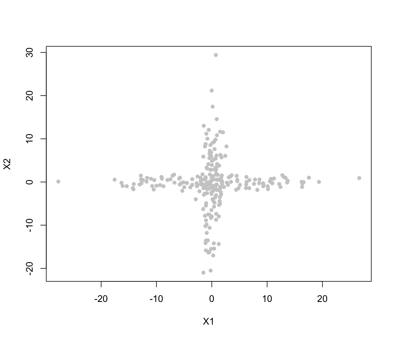
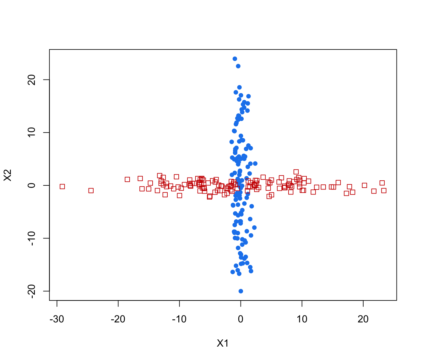
 plot(crossMclustDA, what = "classification")
 plot(crossMclustDA, what = "classification", newdata = cross[even,-1])
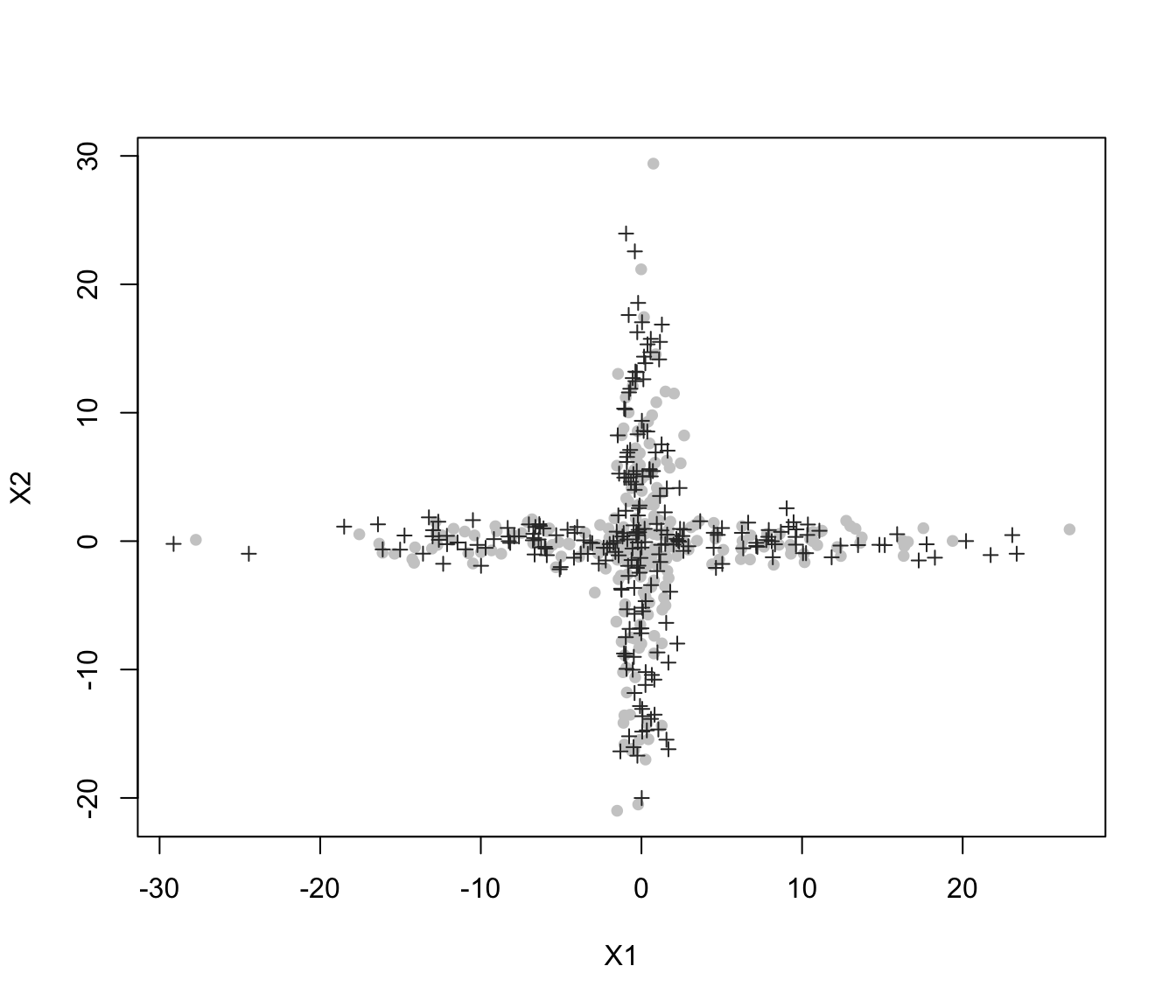
 plot(crossMclustDA, what = "train&test", newdata = cross[even,-1])
 plot(crossMclustDA, what = "error")
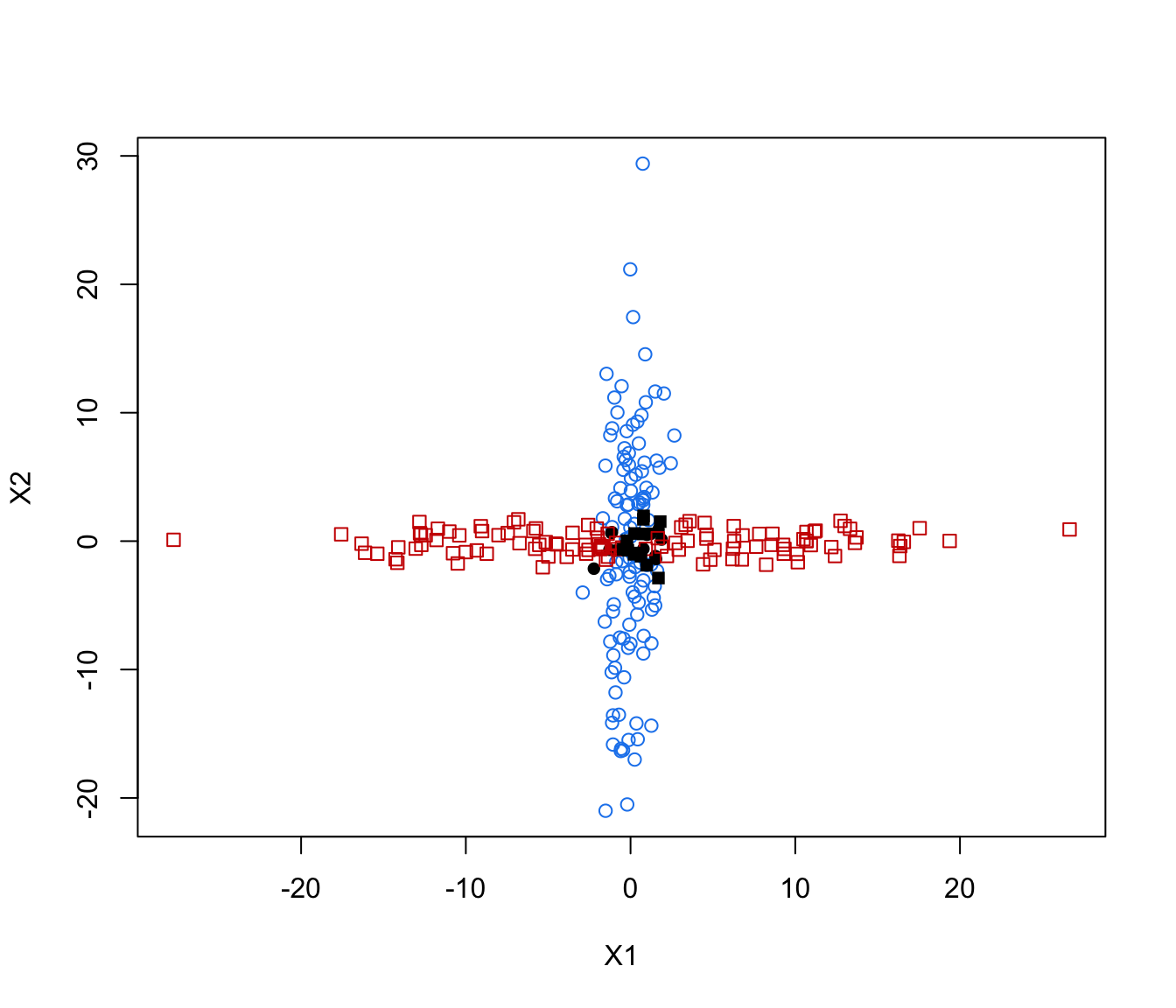 plot(crossMclustDA, what = "error", newdata =cross[even,-1], newclass = cross[even,1])
 # }
# }