Estimation of class prior probabilities by EM algorithm
classPriorProbs.RdA simple procedure to improve the estimation of class prior probabilities when the training data does not reflect the true a priori probabilities of the target classes. The EM algorithm used is described in Saerens et al (2002).
Usage
classPriorProbs(object, newdata = object$data,
                itmax = 1e3, eps = sqrt(.Machine$double.eps))
Arguments
- object
an object of class
'MclustDA'resulting from a call toMclustDA.- newdata
a data frame or matrix giving the data. If missing the train data obtained from the call to
MclustDAare used.- itmax
an integer value specifying the maximal number of EM iterations.
- eps
a scalar specifying the tolerance associated with deciding when to terminate the EM iterations.
Value
A vector of class prior estimates which can then be used in the predict.MclustDA to improve predictions.
References
Saerens, M., Latinne, P. and Decaestecker, C. (2002) Adjusting the outputs of a classifier to new a priori probabilities: a simple procedure, Neural computation, 14 (1), 21–41.
Examples
# \donttest{
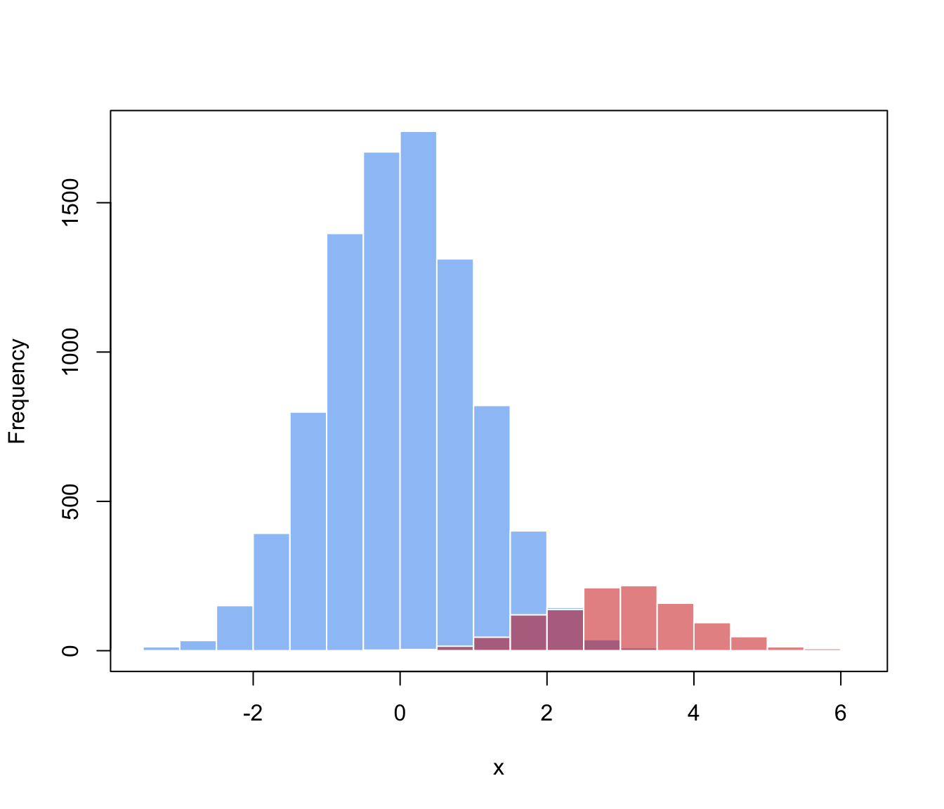
# generate data from a mixture f(x) = 0.9 * N(0,1) + 0.1 * N(3,1)
n <- 10000
mixpro <- c(0.9, 0.1)
class <- factor(sample(0:1, size = n, prob = mixpro, replace = TRUE))
x <- ifelse(class == 1, rnorm(n, mean = 3, sd = 1),
rnorm(n, mean = 0, sd = 1))
hist(x[class==0], breaks = 11, xlim = range(x), main = "", xlab = "x",
col = adjustcolor("dodgerblue2", alpha.f = 0.5), border = "white")
hist(x[class==1], breaks = 11, add = TRUE,
col = adjustcolor("red3", alpha.f = 0.5), border = "white")
box()
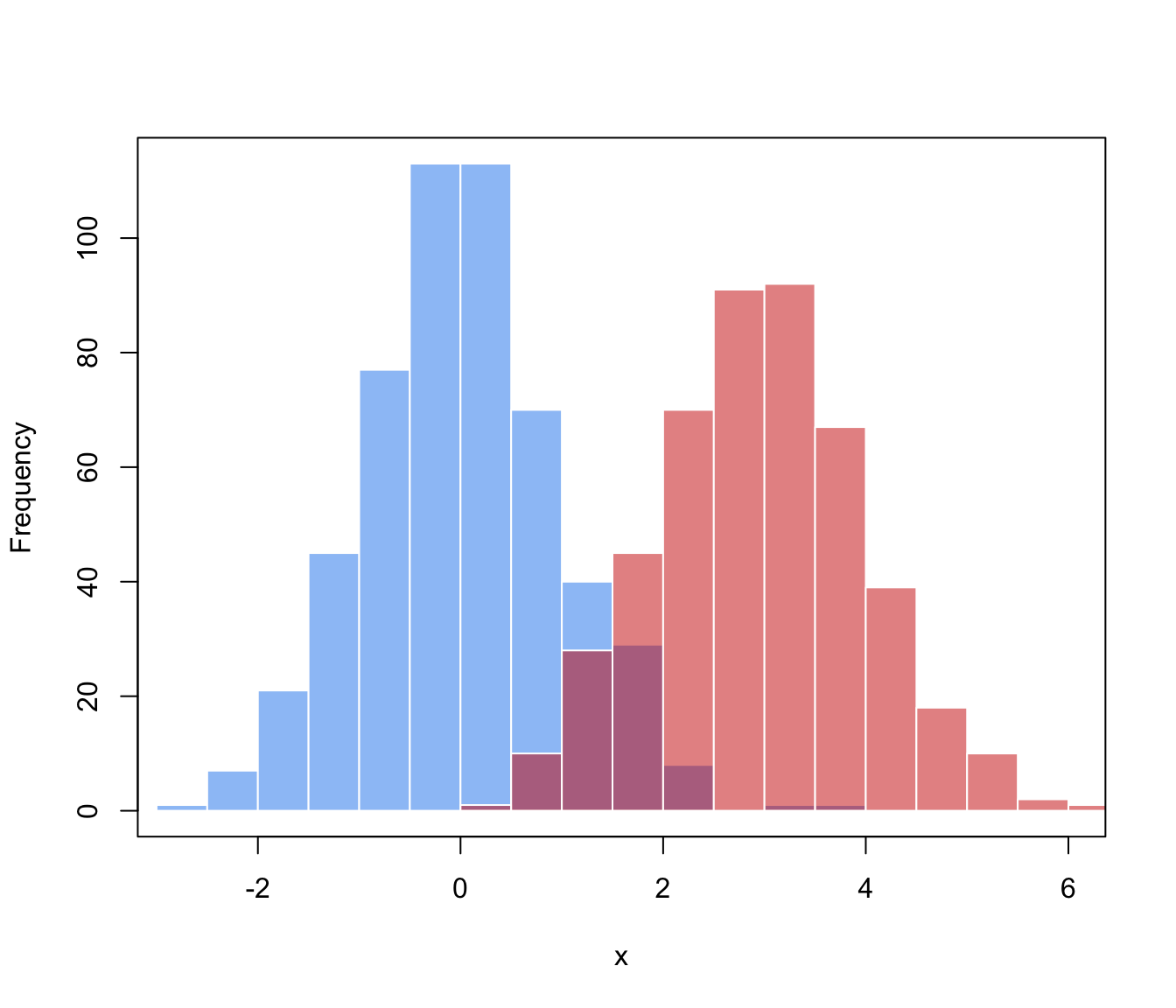
 # generate training data from a balanced case-control sample, i.e.
# f(x) = 0.5 * N(0,1) + 0.5 * N(3,1)
n_train <- 1000
class_train <- factor(sample(0:1, size = n_train, prob = c(0.5, 0.5), replace = TRUE))
x_train <- ifelse(class_train == 1, rnorm(n_train, mean = 3, sd = 1),
rnorm(n_train, mean = 0, sd = 1))
hist(x_train[class_train==0], breaks = 11, xlim = range(x_train),
main = "", xlab = "x",
col = adjustcolor("dodgerblue2", alpha.f = 0.5), border = "white")
hist(x_train[class_train==1], breaks = 11, add = TRUE,
col = adjustcolor("red3", alpha.f = 0.5), border = "white")
box()
# generate training data from a balanced case-control sample, i.e.
# f(x) = 0.5 * N(0,1) + 0.5 * N(3,1)
n_train <- 1000
class_train <- factor(sample(0:1, size = n_train, prob = c(0.5, 0.5), replace = TRUE))
x_train <- ifelse(class_train == 1, rnorm(n_train, mean = 3, sd = 1),
rnorm(n_train, mean = 0, sd = 1))
hist(x_train[class_train==0], breaks = 11, xlim = range(x_train),
main = "", xlab = "x",
col = adjustcolor("dodgerblue2", alpha.f = 0.5), border = "white")
hist(x_train[class_train==1], breaks = 11, add = TRUE,
col = adjustcolor("red3", alpha.f = 0.5), border = "white")
box()
 # fit a MclustDA model
mod <- MclustDA(x_train, class_train)
summary(mod, parameters = TRUE)
#> ------------------------------------------------
#> Gaussian finite mixture model for classification
#> ------------------------------------------------
#>
#> MclustDA
#> ------------------------------------------------
#> log-likelihood n df BIC
#> -1919.962 1000 5 -3874.463
#>
#> Classes n % Model G
#> 0 526 52.6 X 1
#> 1 474 47.4 X 1
#>
#> Parameter estimates
#> ------------------------------------------------
#> Class prior probabilities:
#> 0 1
#> 0.526 0.474
#>
#> Class = 0
#> ---------
#>
#> Mixing probabilities: 1
#>
#> Means:
#> [1] 0.02488499
#>
#> Variances:
#> [1] 0.903712
#>
#> Class = 1
#> ---------
#>
#> Mixing probabilities: 1
#>
#> Means:
#> [1] 2.961555
#>
#> Variances:
#> [1] 1.026875
#>
#> Training confusion matrix
#> ------------------------------------------------
#> Predicted
#> Classes 0 1
#> 0 487 39
#> 1 40 434
#>
#> Classification error = 0.0790
#> Brier score = 0.0514
# test set performance
pred <- predict(mod, newdata = x)
classError(pred$classification, class)$error
#> [1] 0.0659
BrierScore(pred$z, class)
#> [1] 0.04868675
# compute performance over a grid of prior probs
priorProp <- seq(0.01, 0.99, by = 0.01)
CE <- BS <- rep(as.double(NA), length(priorProp))
for(i in seq(priorProp))
{
pred <- predict(mod, newdata = x, prop = c(1-priorProp[i], priorProp[i]))
CE[i] <- classError(pred$classification, class = class)$error
BS[i] <- BrierScore(pred$z, class)
}
# estimate the optimal class prior probs
(priorProbs <- classPriorProbs(mod, x))
#> 0 1
#> 0.8877376 0.1122624
pred <- predict(mod, newdata = x, prop = priorProbs)
# compute performance at the estimated class prior probs
classError(pred$classification, class = class)$error
#> [1] 0.0356
BrierScore(pred$z, class)
#> [1] 0.02670998
matplot(priorProp, cbind(CE,BS), type = "l", lty = 1, lwd = 2,
xlab = "Class prior probability", ylab = "", ylim = c(0,max(CE,BS)),
panel.first =
{ abline(h = seq(0,1,by=0.05), col = "grey", lty = 3)
abline(v = seq(0,1,by=0.05), col = "grey", lty = 3)
})
abline(v = mod$prop[2], lty = 2) # training prop
abline(v = mean(class==1), lty = 4) # test prop (usually unknown)
abline(v = priorProbs[2], lty = 3, lwd = 2) # estimated prior probs
legend("topleft", legend = c("ClassError", "BrierScore"),
col = 1:2, lty = 1, lwd = 2, inset = 0.02)
# fit a MclustDA model
mod <- MclustDA(x_train, class_train)
summary(mod, parameters = TRUE)
#> ------------------------------------------------
#> Gaussian finite mixture model for classification
#> ------------------------------------------------
#>
#> MclustDA
#> ------------------------------------------------
#> log-likelihood n df BIC
#> -1919.962 1000 5 -3874.463
#>
#> Classes n % Model G
#> 0 526 52.6 X 1
#> 1 474 47.4 X 1
#>
#> Parameter estimates
#> ------------------------------------------------
#> Class prior probabilities:
#> 0 1
#> 0.526 0.474
#>
#> Class = 0
#> ---------
#>
#> Mixing probabilities: 1
#>
#> Means:
#> [1] 0.02488499
#>
#> Variances:
#> [1] 0.903712
#>
#> Class = 1
#> ---------
#>
#> Mixing probabilities: 1
#>
#> Means:
#> [1] 2.961555
#>
#> Variances:
#> [1] 1.026875
#>
#> Training confusion matrix
#> ------------------------------------------------
#> Predicted
#> Classes 0 1
#> 0 487 39
#> 1 40 434
#>
#> Classification error = 0.0790
#> Brier score = 0.0514
# test set performance
pred <- predict(mod, newdata = x)
classError(pred$classification, class)$error
#> [1] 0.0659
BrierScore(pred$z, class)
#> [1] 0.04868675
# compute performance over a grid of prior probs
priorProp <- seq(0.01, 0.99, by = 0.01)
CE <- BS <- rep(as.double(NA), length(priorProp))
for(i in seq(priorProp))
{
pred <- predict(mod, newdata = x, prop = c(1-priorProp[i], priorProp[i]))
CE[i] <- classError(pred$classification, class = class)$error
BS[i] <- BrierScore(pred$z, class)
}
# estimate the optimal class prior probs
(priorProbs <- classPriorProbs(mod, x))
#> 0 1
#> 0.8877376 0.1122624
pred <- predict(mod, newdata = x, prop = priorProbs)
# compute performance at the estimated class prior probs
classError(pred$classification, class = class)$error
#> [1] 0.0356
BrierScore(pred$z, class)
#> [1] 0.02670998
matplot(priorProp, cbind(CE,BS), type = "l", lty = 1, lwd = 2,
xlab = "Class prior probability", ylab = "", ylim = c(0,max(CE,BS)),
panel.first =
{ abline(h = seq(0,1,by=0.05), col = "grey", lty = 3)
abline(v = seq(0,1,by=0.05), col = "grey", lty = 3)
})
abline(v = mod$prop[2], lty = 2) # training prop
abline(v = mean(class==1), lty = 4) # test prop (usually unknown)
abline(v = priorProbs[2], lty = 3, lwd = 2) # estimated prior probs
legend("topleft", legend = c("ClassError", "BrierScore"),
col = 1:2, lty = 1, lwd = 2, inset = 0.02)
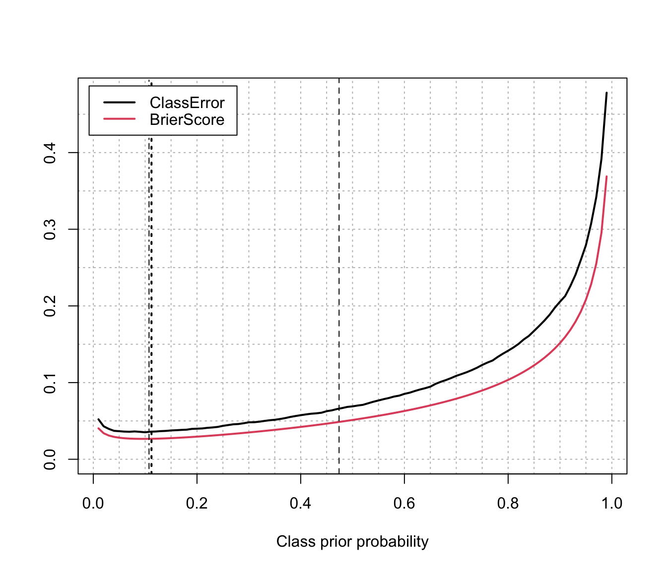 # Summary of results:
priorProp[which.min(CE)] # best prior of class 1 according to classification error
#> [1] 0.1
priorProp[which.min(BS)] # best prior of class 1 according to Brier score
#> [1] 0.1
priorProbs # optimal estimated class prior probabilities
#> 0 1
#> 0.8877376 0.1122624
# }
# Summary of results:
priorProp[which.min(CE)] # best prior of class 1 according to classification error
#> [1] 0.1
priorProp[which.min(BS)] # best prior of class 1 according to Brier score
#> [1] 0.1
priorProbs # optimal estimated class prior probabilities
#> 0 1
#> 0.8877376 0.1122624
# }