Density Estimation via Model-Based Clustering
densityMclust.RdProduces a density estimate for each data point using a Gaussian finite
mixture model from Mclust.
Arguments
- data
A numeric vector, matrix, or data frame of observations. Categorical variables are not allowed. If a matrix or data frame, rows correspond to observations and columns correspond to variables.
- ...
Additional arguments for the
Mclustfunction. In particular, setting the argumentsGandmodelNamesallow to specify the number of mixture components and the type of model to be fitted. By default an "optimal" model is selected based on the BIC criterion.- plot
A logical value specifying if the estimated density should be plotted. For more contols on the resulting graph see the associated
plot.densityMclustmethod.
Value
An object of class densityMclust, which inherits from
Mclust. This contains all the components described in
Mclust and the additional element:
- density
The density evaluated at the input
datacomputed from the estimated model.
References
Scrucca L., Fraley C., Murphy T. B. and Raftery A. E. (2023) Model-Based Clustering, Classification, and Density Estimation Using mclust in R. Chapman & Hall/CRC, ISBN: 978-1032234953, https://mclust-org.github.io/book/
Scrucca L., Fop M., Murphy T. B. and Raftery A. E. (2016) mclust 5: clustering, classification and density estimation using Gaussian finite mixture models, The R Journal, 8/1, pp. 289-317.
Fraley C. and Raftery A. E. (2002) Model-based clustering, discriminant analysis and density estimation, Journal of the American Statistical Association, 97/458, pp. 611-631.
Examples
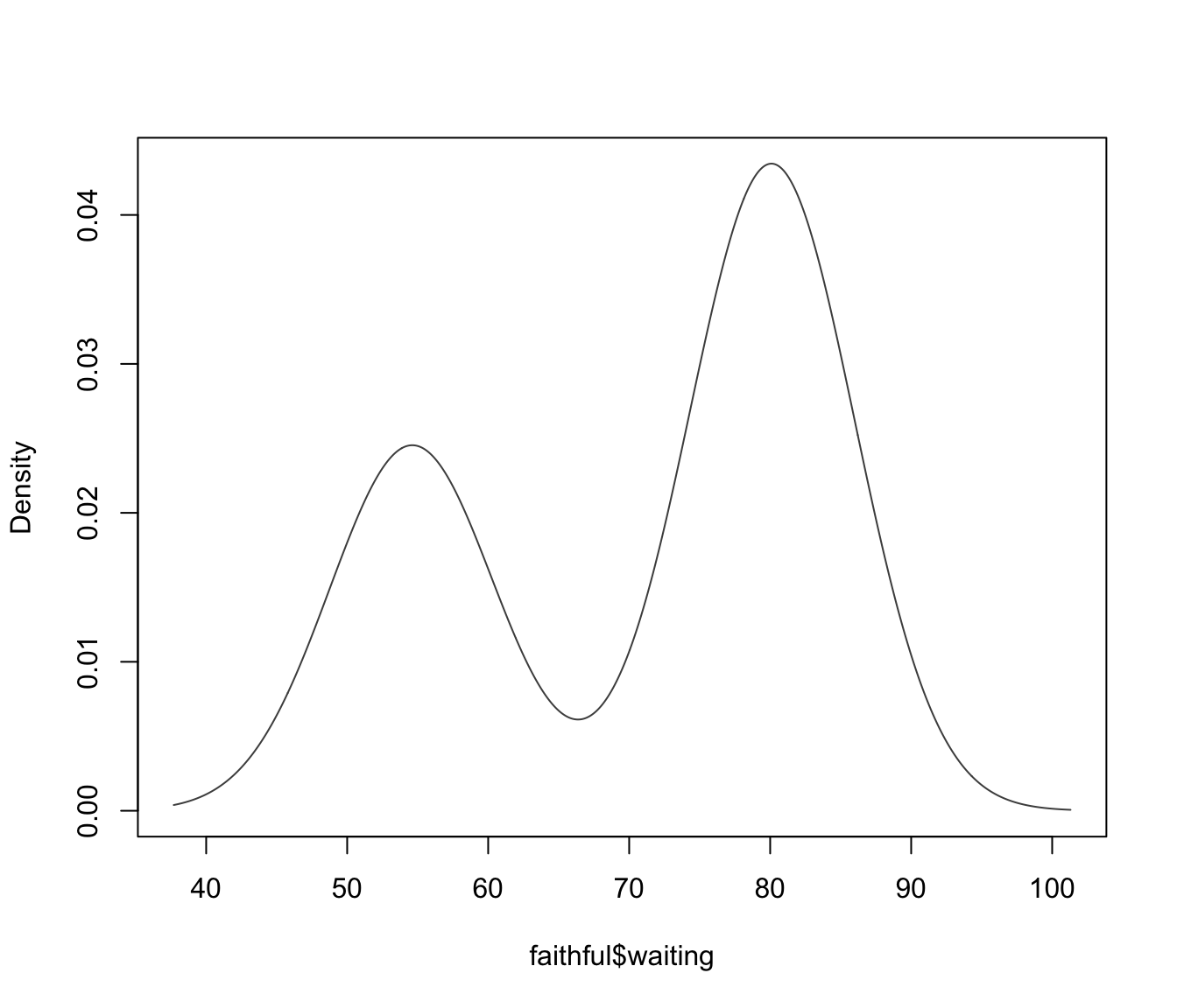
dens <- densityMclust(faithful$waiting)
 summary(dens)
#> -------------------------------------------------------
#> Density estimation via Gaussian finite mixture modeling
#> -------------------------------------------------------
#>
#> Mclust E (univariate, equal variance) model with 2 components:
#>
#> log-likelihood n df BIC ICL
#> -1034.002 272 4 -2090.427 -2099.576
summary(dens, parameters = TRUE)
#> -------------------------------------------------------
#> Density estimation via Gaussian finite mixture modeling
#> -------------------------------------------------------
#>
#> Mclust E (univariate, equal variance) model with 2 components:
#>
#> log-likelihood n df BIC ICL
#> -1034.002 272 4 -2090.427 -2099.576
#>
#> Mixing probabilities:
#> 1 2
#> 0.3609461 0.6390539
#>
#> Means:
#> 1 2
#> 54.61675 80.09239
#>
#> Variances:
#> 1 2
#> 34.44093 34.44093
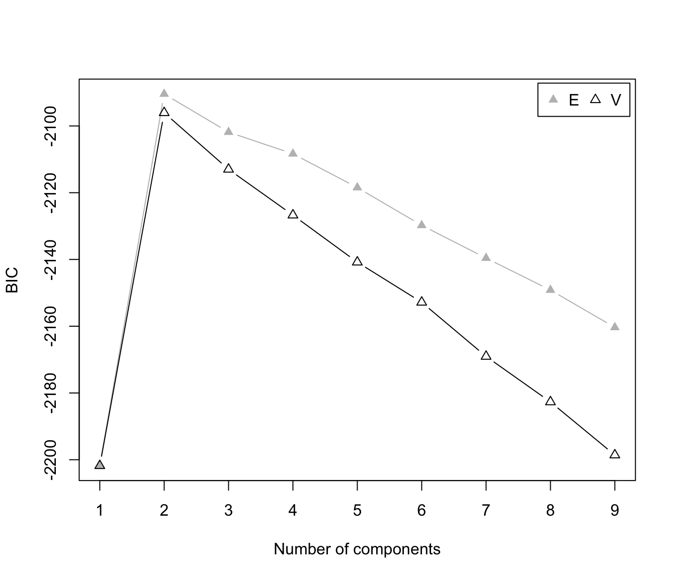
plot(dens, what = "BIC", legendArgs = list(x = "topright"))
summary(dens)
#> -------------------------------------------------------
#> Density estimation via Gaussian finite mixture modeling
#> -------------------------------------------------------
#>
#> Mclust E (univariate, equal variance) model with 2 components:
#>
#> log-likelihood n df BIC ICL
#> -1034.002 272 4 -2090.427 -2099.576
summary(dens, parameters = TRUE)
#> -------------------------------------------------------
#> Density estimation via Gaussian finite mixture modeling
#> -------------------------------------------------------
#>
#> Mclust E (univariate, equal variance) model with 2 components:
#>
#> log-likelihood n df BIC ICL
#> -1034.002 272 4 -2090.427 -2099.576
#>
#> Mixing probabilities:
#> 1 2
#> 0.3609461 0.6390539
#>
#> Means:
#> 1 2
#> 54.61675 80.09239
#>
#> Variances:
#> 1 2
#> 34.44093 34.44093
plot(dens, what = "BIC", legendArgs = list(x = "topright"))
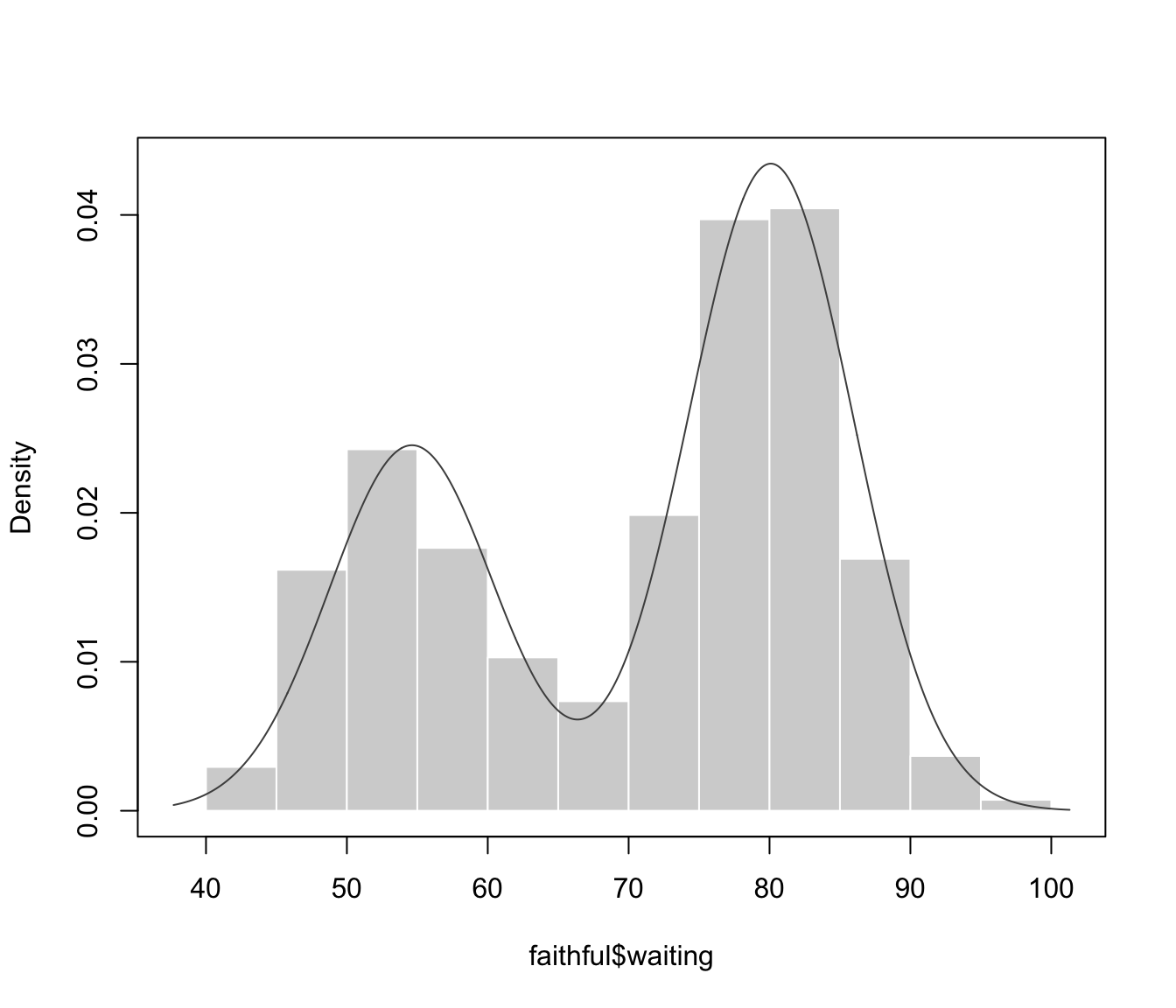
 plot(dens, what = "density", data = faithful$waiting)
 dens <- densityMclust(faithful, modelNames = "EEE", G = 3, plot = FALSE)
summary(dens)
#> -------------------------------------------------------
#> Density estimation via Gaussian finite mixture modeling
#> -------------------------------------------------------
#>
#> Mclust EEE (ellipsoidal, equal volume, shape and orientation) model with 3
#> components:
#>
#> log-likelihood n df BIC ICL
#> -1126.326 272 11 -2314.316 -2357.824
summary(dens, parameters = TRUE)
#> -------------------------------------------------------
#> Density estimation via Gaussian finite mixture modeling
#> -------------------------------------------------------
#>
#> Mclust EEE (ellipsoidal, equal volume, shape and orientation) model with 3
#> components:
#>
#> log-likelihood n df BIC ICL
#> -1126.326 272 11 -2314.316 -2357.824
#>
#> Mixing probabilities:
#> 1 2 3
#> 0.1656784 0.3563696 0.4779520
#>
#> Means:
#> [,1] [,2] [,3]
#> eruptions 3.793066 2.037596 4.463245
#> waiting 77.521051 54.491158 80.833439
#>
#> Variances:
#> [,,1]
#> eruptions waiting
#> eruptions 0.07825448 0.4801979
#> waiting 0.48019785 33.7671464
#> [,,2]
#> eruptions waiting
#> eruptions 0.07825448 0.4801979
#> waiting 0.48019785 33.7671464
#> [,,3]
#> eruptions waiting
#> eruptions 0.07825448 0.4801979
#> waiting 0.48019785 33.7671464
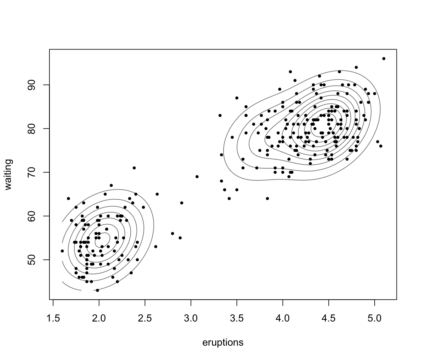
plot(dens, what = "density", data = faithful,
drawlabels = FALSE, points.pch = 20)
dens <- densityMclust(faithful, modelNames = "EEE", G = 3, plot = FALSE)
summary(dens)
#> -------------------------------------------------------
#> Density estimation via Gaussian finite mixture modeling
#> -------------------------------------------------------
#>
#> Mclust EEE (ellipsoidal, equal volume, shape and orientation) model with 3
#> components:
#>
#> log-likelihood n df BIC ICL
#> -1126.326 272 11 -2314.316 -2357.824
summary(dens, parameters = TRUE)
#> -------------------------------------------------------
#> Density estimation via Gaussian finite mixture modeling
#> -------------------------------------------------------
#>
#> Mclust EEE (ellipsoidal, equal volume, shape and orientation) model with 3
#> components:
#>
#> log-likelihood n df BIC ICL
#> -1126.326 272 11 -2314.316 -2357.824
#>
#> Mixing probabilities:
#> 1 2 3
#> 0.1656784 0.3563696 0.4779520
#>
#> Means:
#> [,1] [,2] [,3]
#> eruptions 3.793066 2.037596 4.463245
#> waiting 77.521051 54.491158 80.833439
#>
#> Variances:
#> [,,1]
#> eruptions waiting
#> eruptions 0.07825448 0.4801979
#> waiting 0.48019785 33.7671464
#> [,,2]
#> eruptions waiting
#> eruptions 0.07825448 0.4801979
#> waiting 0.48019785 33.7671464
#> [,,3]
#> eruptions waiting
#> eruptions 0.07825448 0.4801979
#> waiting 0.48019785 33.7671464
plot(dens, what = "density", data = faithful,
drawlabels = FALSE, points.pch = 20)
 plot(dens, what = "density", type = "hdr")
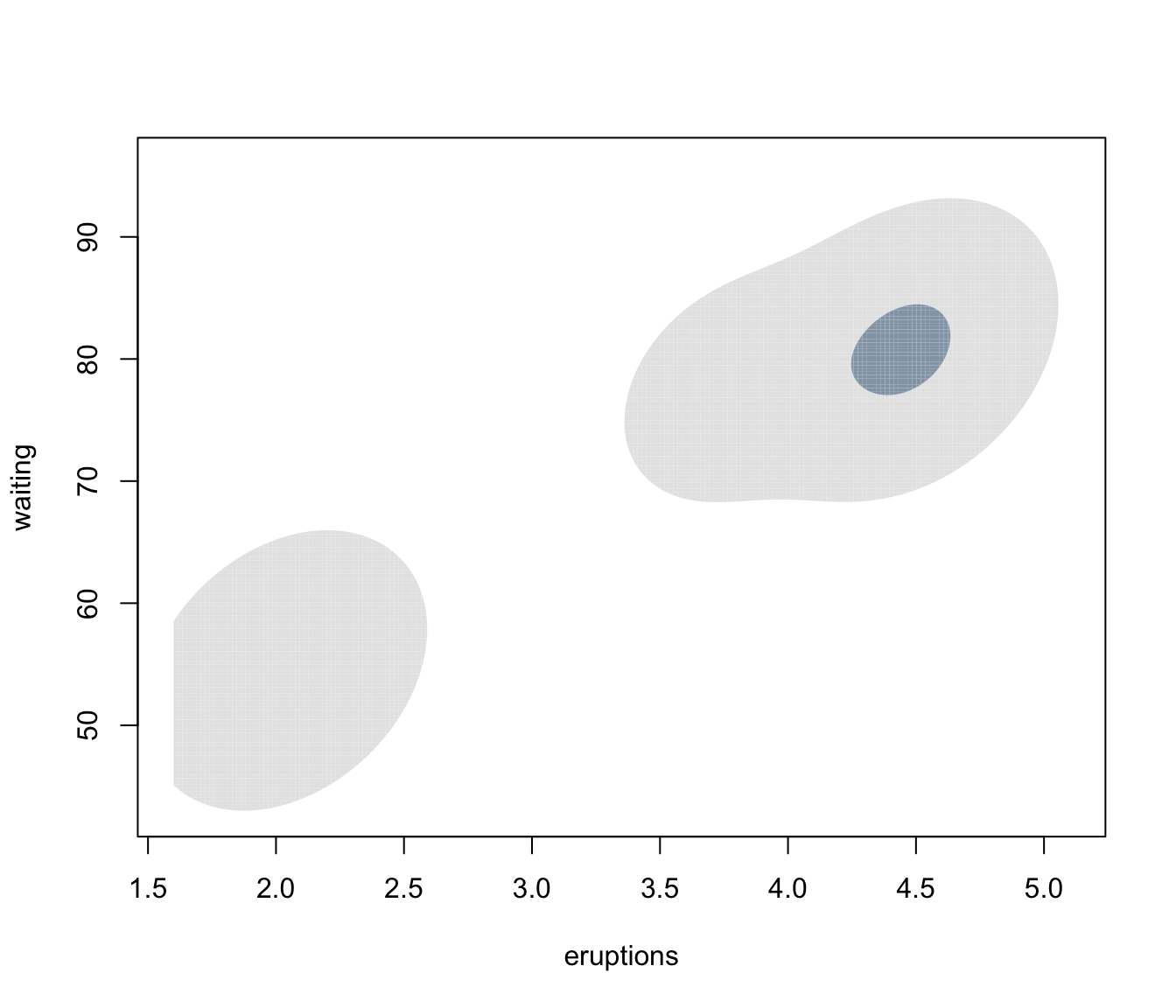
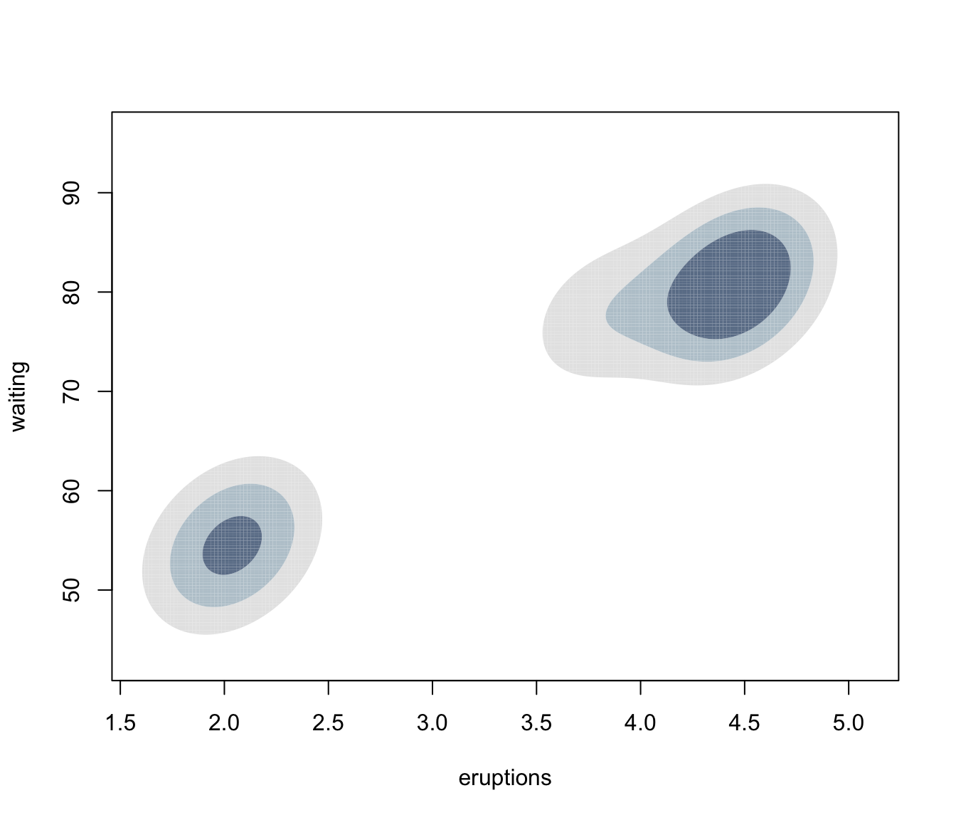 plot(dens, what = "density", type = "hdr", prob = c(0.1, 0.9))
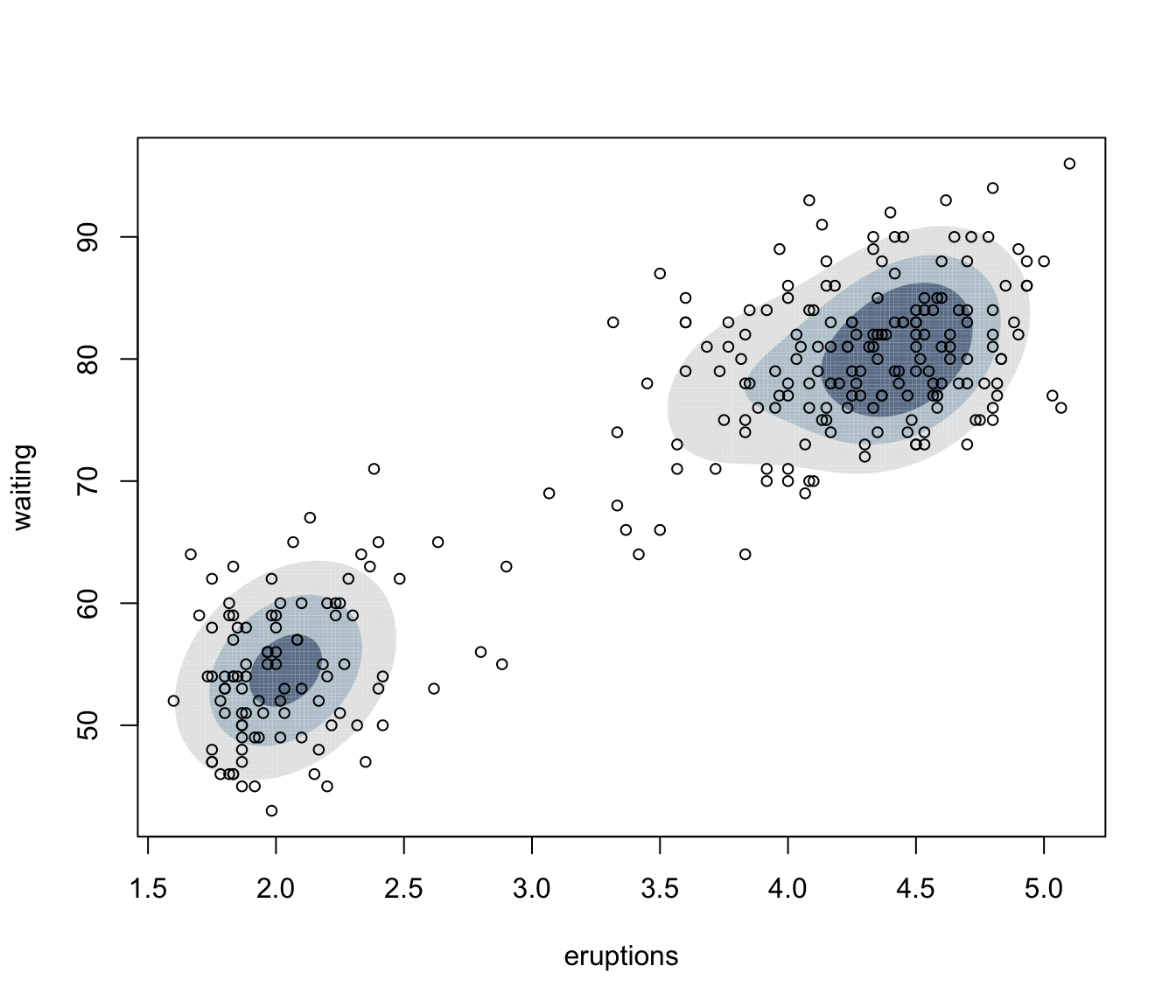
 plot(dens, what = "density", type = "hdr", data = faithful)
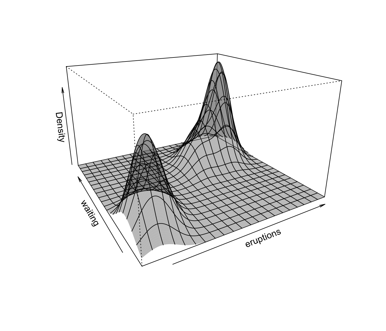
 plot(dens, what = "density", type = "persp")
 # \donttest{
dens <- densityMclust(iris[,1:4], G = 2)
# \donttest{
dens <- densityMclust(iris[,1:4], G = 2)
 summary(dens, parameters = TRUE)
#> -------------------------------------------------------
#> Density estimation via Gaussian finite mixture modeling
#> -------------------------------------------------------
#>
#> Mclust VEV (ellipsoidal, equal shape) model with 2 components:
#>
#> log-likelihood n df BIC ICL
#> -215.726 150 26 -561.7285 -561.7289
#>
#> Mixing probabilities:
#> 1 2
#> 0.3333319 0.6666681
#>
#> Means:
#> [,1] [,2]
#> Sepal.Length 5.0060022 6.261996
#> Sepal.Width 3.4280049 2.871999
#> Petal.Length 1.4620007 4.905992
#> Petal.Width 0.2459998 1.675997
#>
#> Variances:
#> [,,1]
#> Sepal.Length Sepal.Width Petal.Length Petal.Width
#> Sepal.Length 0.15065114 0.13080115 0.02084463 0.01309107
#> Sepal.Width 0.13080115 0.17604529 0.01603245 0.01221458
#> Petal.Length 0.02084463 0.01603245 0.02808260 0.00601568
#> Petal.Width 0.01309107 0.01221458 0.00601568 0.01042365
#> [,,2]
#> Sepal.Length Sepal.Width Petal.Length Petal.Width
#> Sepal.Length 0.4000438 0.10865444 0.3994018 0.14368256
#> Sepal.Width 0.1086544 0.10928077 0.1238904 0.07284384
#> Petal.Length 0.3994018 0.12389040 0.6109024 0.25738990
#> Petal.Width 0.1436826 0.07284384 0.2573899 0.16808182
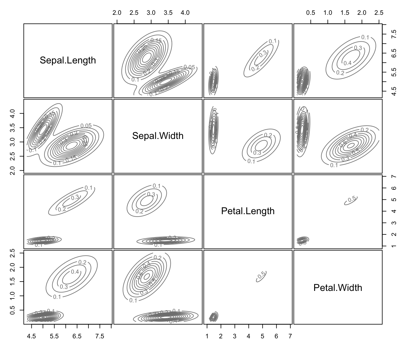
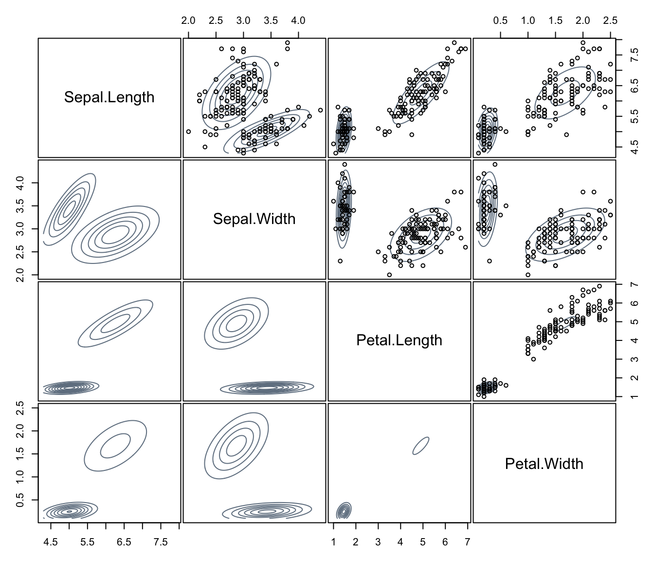
plot(dens, what = "density", data = iris[,1:4],
col = "slategrey", drawlabels = FALSE, nlevels = 7)
summary(dens, parameters = TRUE)
#> -------------------------------------------------------
#> Density estimation via Gaussian finite mixture modeling
#> -------------------------------------------------------
#>
#> Mclust VEV (ellipsoidal, equal shape) model with 2 components:
#>
#> log-likelihood n df BIC ICL
#> -215.726 150 26 -561.7285 -561.7289
#>
#> Mixing probabilities:
#> 1 2
#> 0.3333319 0.6666681
#>
#> Means:
#> [,1] [,2]
#> Sepal.Length 5.0060022 6.261996
#> Sepal.Width 3.4280049 2.871999
#> Petal.Length 1.4620007 4.905992
#> Petal.Width 0.2459998 1.675997
#>
#> Variances:
#> [,,1]
#> Sepal.Length Sepal.Width Petal.Length Petal.Width
#> Sepal.Length 0.15065114 0.13080115 0.02084463 0.01309107
#> Sepal.Width 0.13080115 0.17604529 0.01603245 0.01221458
#> Petal.Length 0.02084463 0.01603245 0.02808260 0.00601568
#> Petal.Width 0.01309107 0.01221458 0.00601568 0.01042365
#> [,,2]
#> Sepal.Length Sepal.Width Petal.Length Petal.Width
#> Sepal.Length 0.4000438 0.10865444 0.3994018 0.14368256
#> Sepal.Width 0.1086544 0.10928077 0.1238904 0.07284384
#> Petal.Length 0.3994018 0.12389040 0.6109024 0.25738990
#> Petal.Width 0.1436826 0.07284384 0.2573899 0.16808182
plot(dens, what = "density", data = iris[,1:4],
col = "slategrey", drawlabels = FALSE, nlevels = 7)
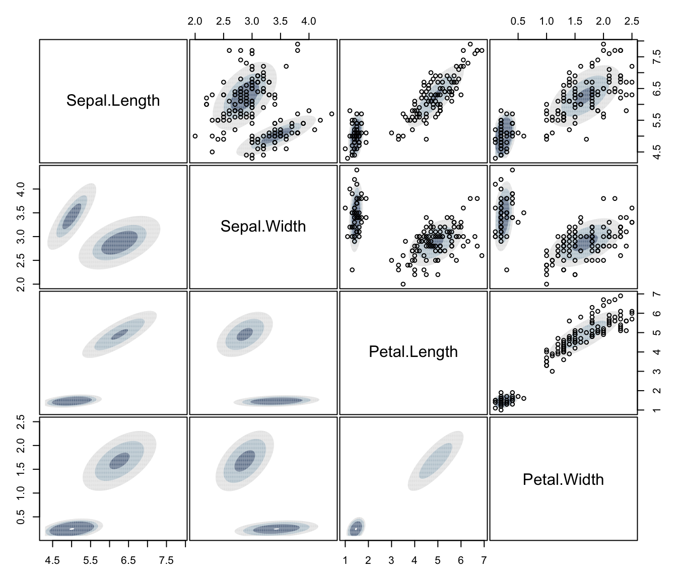
 plot(dens, what = "density", type = "hdr", data = iris[,1:4])
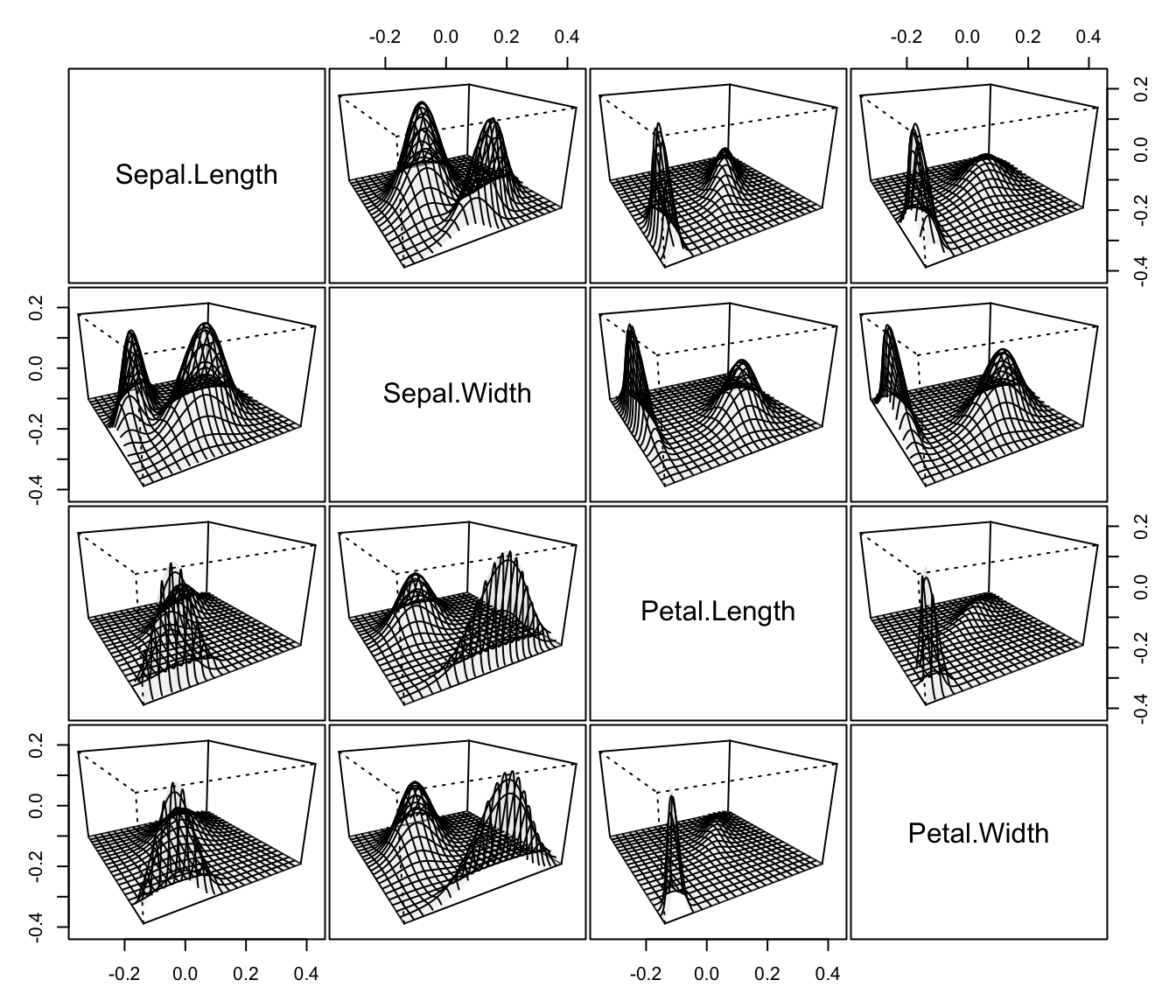
 plot(dens, what = "density", type = "persp", col = grey(0.9))
 # }
# }