Plots for Mixture-Based Density Estimate
plot.densityMclust.RdPlotting methods for an object of class 'mclustDensity'. Available graphs
are plot of BIC values and density for univariate and bivariate data. For
higher data dimensionality a scatterplot matrix of pairwise densities is
drawn.
Usage
# S3 method for class 'densityMclust'
plot(x, data = NULL, what = c("BIC", "density", "diagnostic"), ...)

plotDensityMclust1(x, data = NULL, col = gray(0.3), hist.col = "lightgrey",
                   hist.border = "white",  breaks = "Sturges", ...)

plotDensityMclust2(x, data = NULL, nlevels = 11, levels = NULL,
                   prob = c(0.25, 0.5, 0.75),
                   points.pch = 1, points.col = 1, points.cex = 0.8, ...)

plotDensityMclustd(x, data = NULL, nlevels = 11, levels = NULL,
                   prob = c(0.25, 0.5, 0.75),
                   points.pch = 1, points.col = 1, points.cex = 0.8,
                   gap = 0.2, ...)
Arguments
- x
An object of class
'mclustDensity'obtained from a call todensityMclustfunction.- data
Optional data points.
- what
The type of graph requested:
"density"=a plot of estimated density; if
datais also provided the density is plotted over data points (see Details section)."BIC"=a plot of BIC values for the estimated models versus the number of components.
"diagnostic"=diagnostic plots (only available for the one-dimensional case, see
densityMclust.diagnostic)
- col
The color to be used to draw the density line in 1-dimension or contours in higher dimensions.
- hist.col
The color to be used to fill the bars of the histogram.
- hist.border
The color of the border around the bars of the histogram.
- breaks
See the argument in function
hist.- points.pch, points.col, points.cex
The character symbols, colors, and magnification to be used for plotting
datapoints.- nlevels
An integer, the number of levels to be used in plotting contour densities.
- levels
A vector of density levels at which to draw the contour lines.
- prob
A vector of probability levels for computing HDR. Only used if
type = "hdr"and supersede previousnlevelsandlevelsarguments.- gap
Distance between subplots, in margin lines, for the matrix of pairwise scatterplots.
- ...
Additional arguments passed to
surfacePlot.
Details
The function plot.densityMclust allows to obtain the plot of
estimated density or the graph of BIC values for evaluated models.
If what = "density" the produced plot dependes on the dimensionality
of the data.
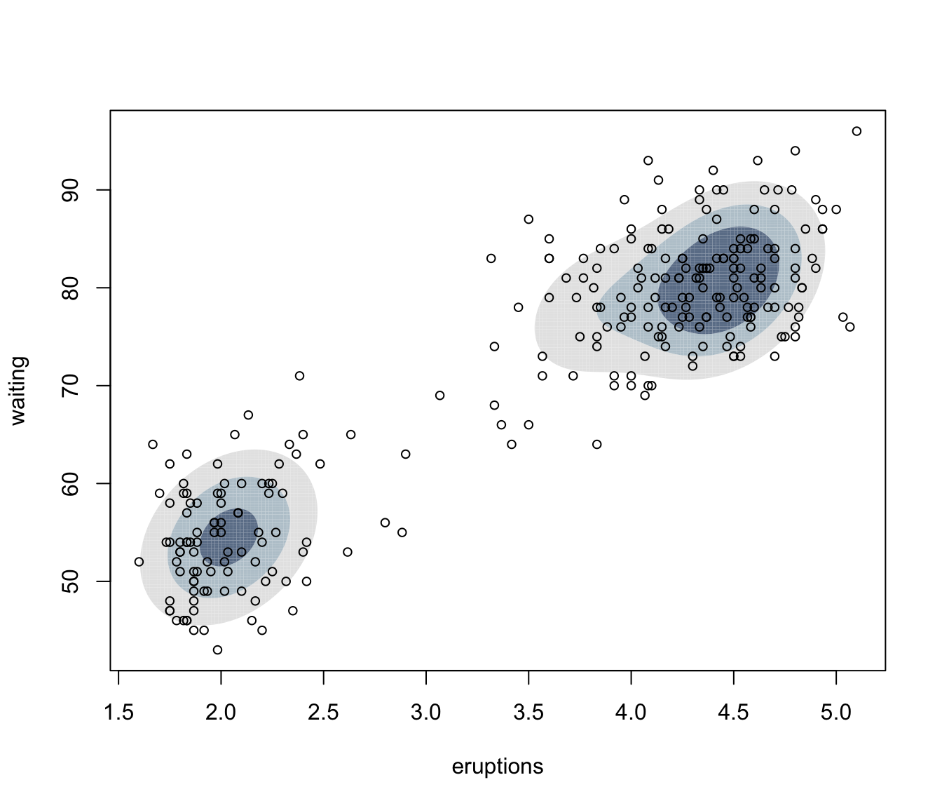
For one-dimensional data a call with no data provided produces a
plot of the estimated density over a sensible range of values. If
data is provided the density is over-plotted on a histogram for the
observed data.
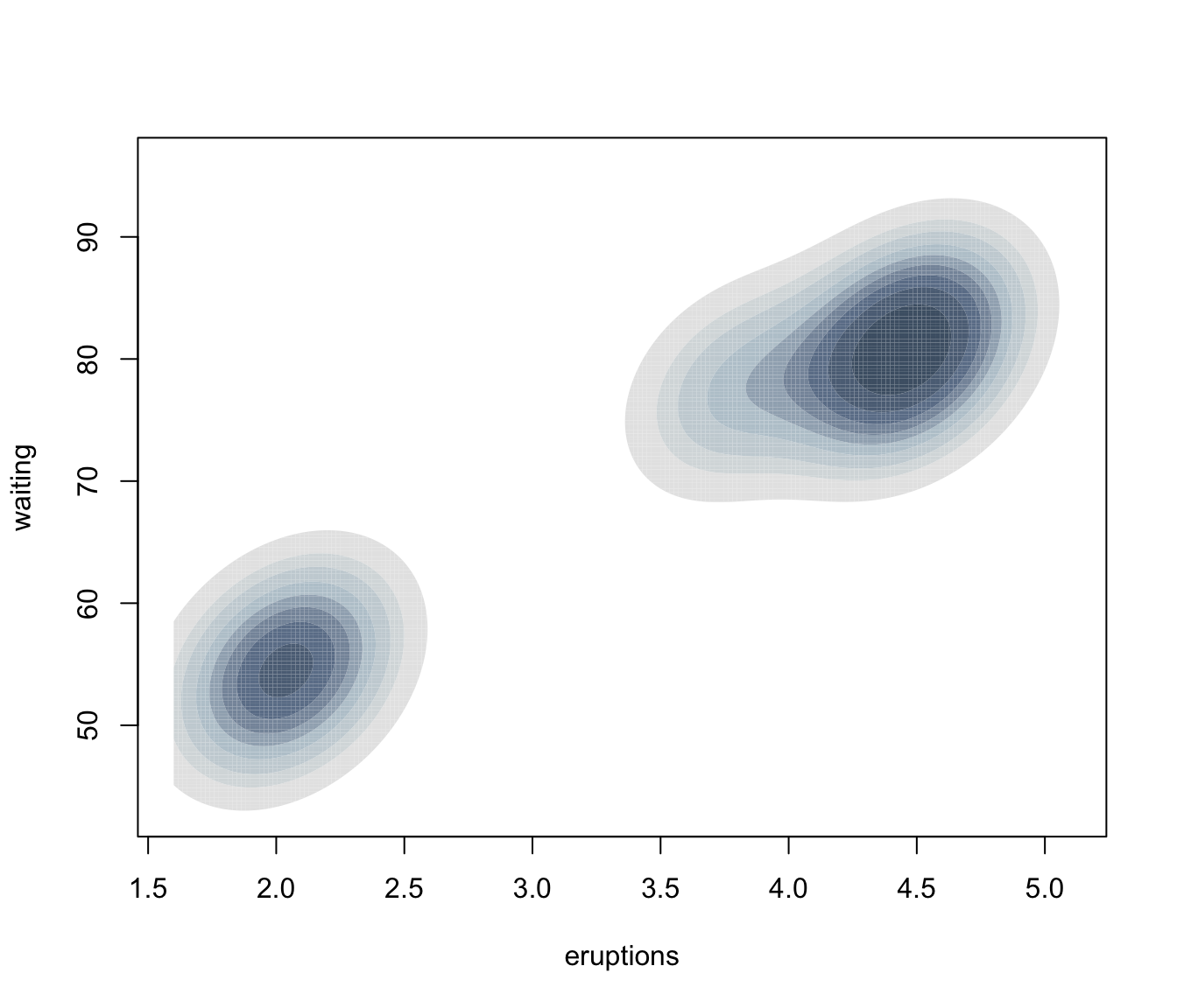
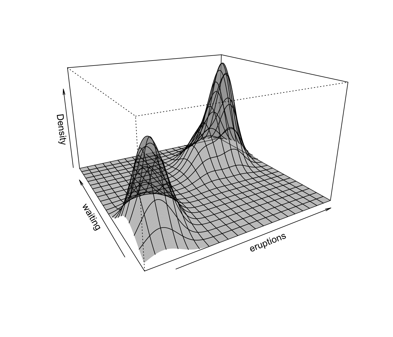
For two-dimensional data further arguments available are those accepted by
the surfacePlot function. In particular, the density can be
represented through "contour", "hdr", "image", and
"persp" type of graph.
For type = "hdr" Highest Density Regions (HDRs) are plotted for
probability levels prob. See hdrlevels for details.
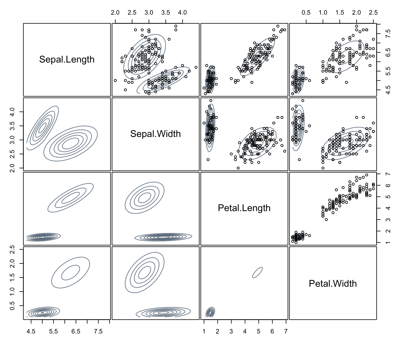
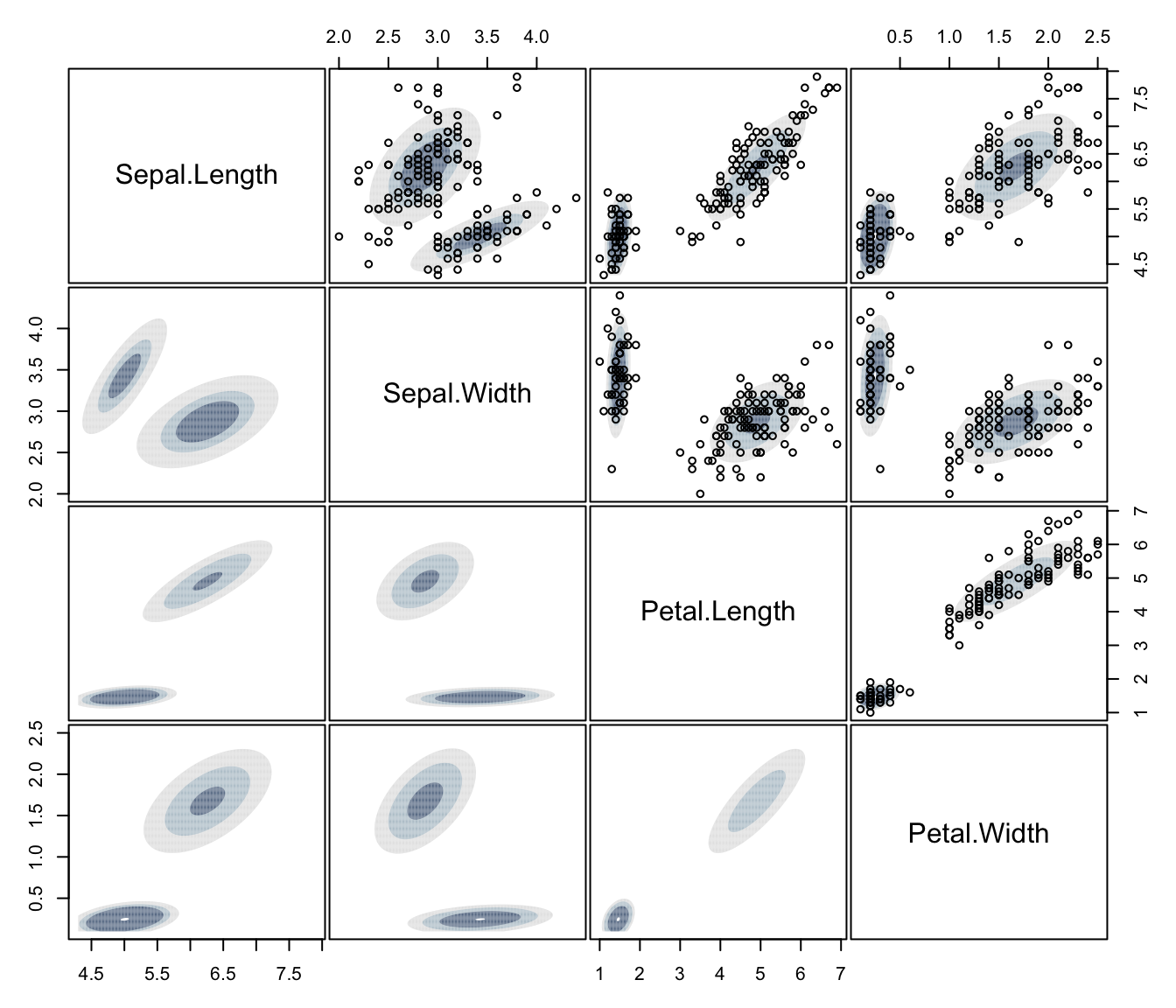
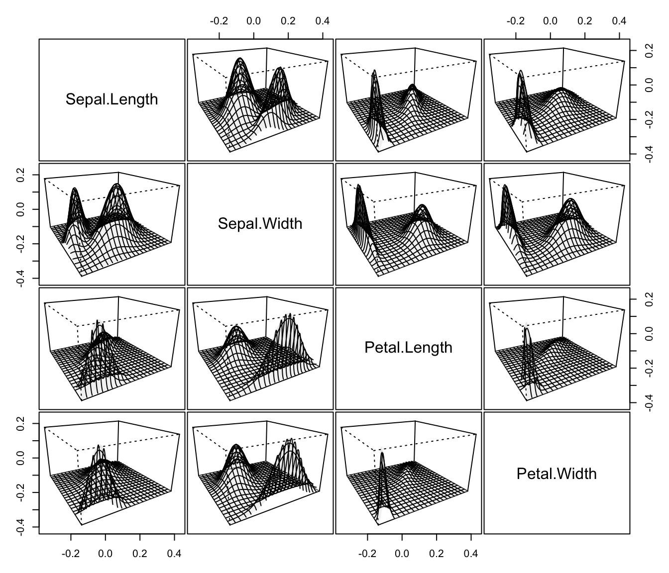
For higher dimensionality a scatterplot matrix of pairwise projected densities is drawn.
Examples
# \donttest{
dens <- densityMclust(faithful$waiting, plot = FALSE)
summary(dens)
#> -------------------------------------------------------
#> Density estimation via Gaussian finite mixture modeling
#> -------------------------------------------------------
#>
#> Mclust E (univariate, equal variance) model with 2 components:
#>
#> log-likelihood n df BIC ICL
#> -1034.002 272 4 -2090.427 -2099.576
summary(dens, parameters = TRUE)
#> -------------------------------------------------------
#> Density estimation via Gaussian finite mixture modeling
#> -------------------------------------------------------
#>
#> Mclust E (univariate, equal variance) model with 2 components:
#>
#> log-likelihood n df BIC ICL
#> -1034.002 272 4 -2090.427 -2099.576
#>
#> Mixing probabilities:
#> 1 2
#> 0.3609461 0.6390539
#>
#> Means:
#> 1 2
#> 54.61675 80.09239
#>
#> Variances:
#> 1 2
#> 34.44093 34.44093
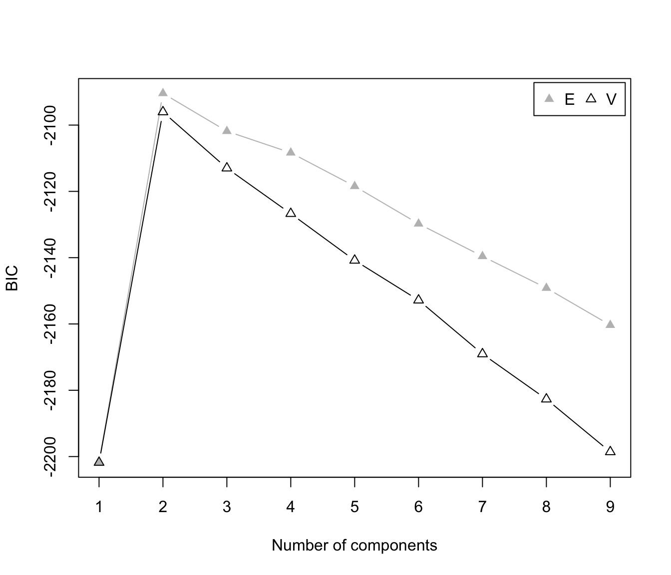
plot(dens, what = "BIC", legendArgs = list(x = "topright"))
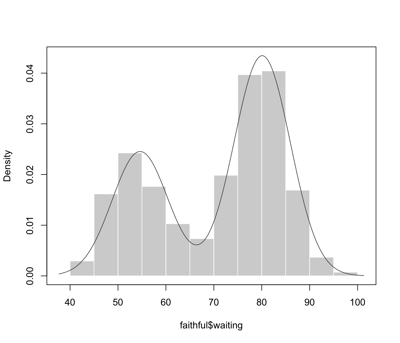
 plot(dens, what = "density", data = faithful$waiting)
 dens <- densityMclust(faithful, plot = FALSE)
summary(dens)
#> -------------------------------------------------------
#> Density estimation via Gaussian finite mixture modeling
#> -------------------------------------------------------
#>
#> Mclust EEE (ellipsoidal, equal volume, shape and orientation) model with 3
#> components:
#>
#> log-likelihood n df BIC ICL
#> -1126.326 272 11 -2314.316 -2357.824
summary(dens, parameters = TRUE)
#> -------------------------------------------------------
#> Density estimation via Gaussian finite mixture modeling
#> -------------------------------------------------------
#>
#> Mclust EEE (ellipsoidal, equal volume, shape and orientation) model with 3
#> components:
#>
#> log-likelihood n df BIC ICL
#> -1126.326 272 11 -2314.316 -2357.824
#>
#> Mixing probabilities:
#> 1 2 3
#> 0.1656784 0.3563696 0.4779520
#>
#> Means:
#> [,1] [,2] [,3]
#> eruptions 3.793066 2.037596 4.463245
#> waiting 77.521051 54.491158 80.833439
#>
#> Variances:
#> [,,1]
#> eruptions waiting
#> eruptions 0.07825448 0.4801979
#> waiting 0.48019785 33.7671464
#> [,,2]
#> eruptions waiting
#> eruptions 0.07825448 0.4801979
#> waiting 0.48019785 33.7671464
#> [,,3]
#> eruptions waiting
#> eruptions 0.07825448 0.4801979
#> waiting 0.48019785 33.7671464
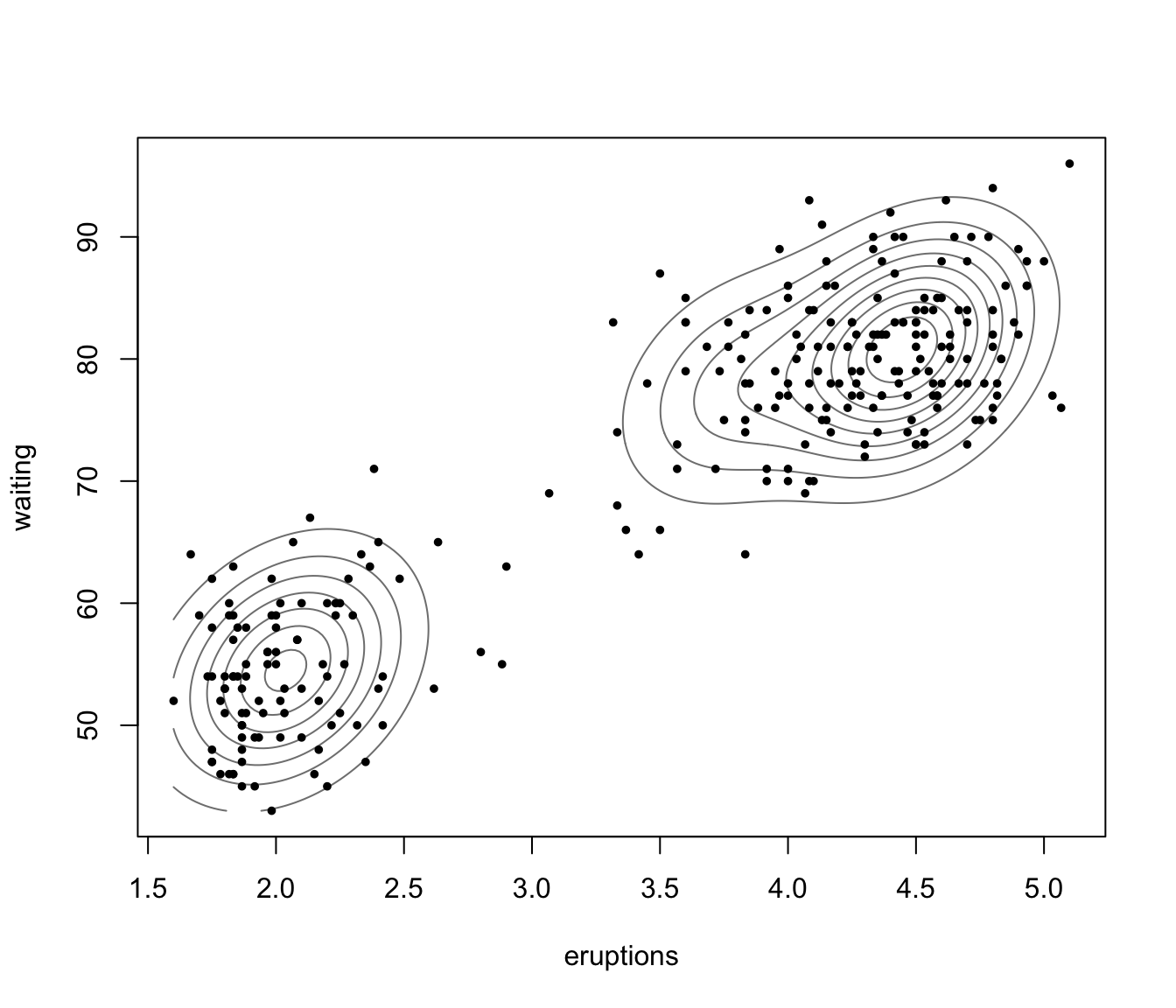
plot(dens, what = "density", data = faithful,
drawlabels = FALSE, points.pch = 20)
dens <- densityMclust(faithful, plot = FALSE)
summary(dens)
#> -------------------------------------------------------
#> Density estimation via Gaussian finite mixture modeling
#> -------------------------------------------------------
#>
#> Mclust EEE (ellipsoidal, equal volume, shape and orientation) model with 3
#> components:
#>
#> log-likelihood n df BIC ICL
#> -1126.326 272 11 -2314.316 -2357.824
summary(dens, parameters = TRUE)
#> -------------------------------------------------------
#> Density estimation via Gaussian finite mixture modeling
#> -------------------------------------------------------
#>
#> Mclust EEE (ellipsoidal, equal volume, shape and orientation) model with 3
#> components:
#>
#> log-likelihood n df BIC ICL
#> -1126.326 272 11 -2314.316 -2357.824
#>
#> Mixing probabilities:
#> 1 2 3
#> 0.1656784 0.3563696 0.4779520
#>
#> Means:
#> [,1] [,2] [,3]
#> eruptions 3.793066 2.037596 4.463245
#> waiting 77.521051 54.491158 80.833439
#>
#> Variances:
#> [,,1]
#> eruptions waiting
#> eruptions 0.07825448 0.4801979
#> waiting 0.48019785 33.7671464
#> [,,2]
#> eruptions waiting
#> eruptions 0.07825448 0.4801979
#> waiting 0.48019785 33.7671464
#> [,,3]
#> eruptions waiting
#> eruptions 0.07825448 0.4801979
#> waiting 0.48019785 33.7671464
plot(dens, what = "density", data = faithful,
drawlabels = FALSE, points.pch = 20)
 plot(dens, what = "density", type = "hdr")
 plot(dens, what = "density", type = "hdr", prob = seq(0.1, 0.9, by = 0.1))
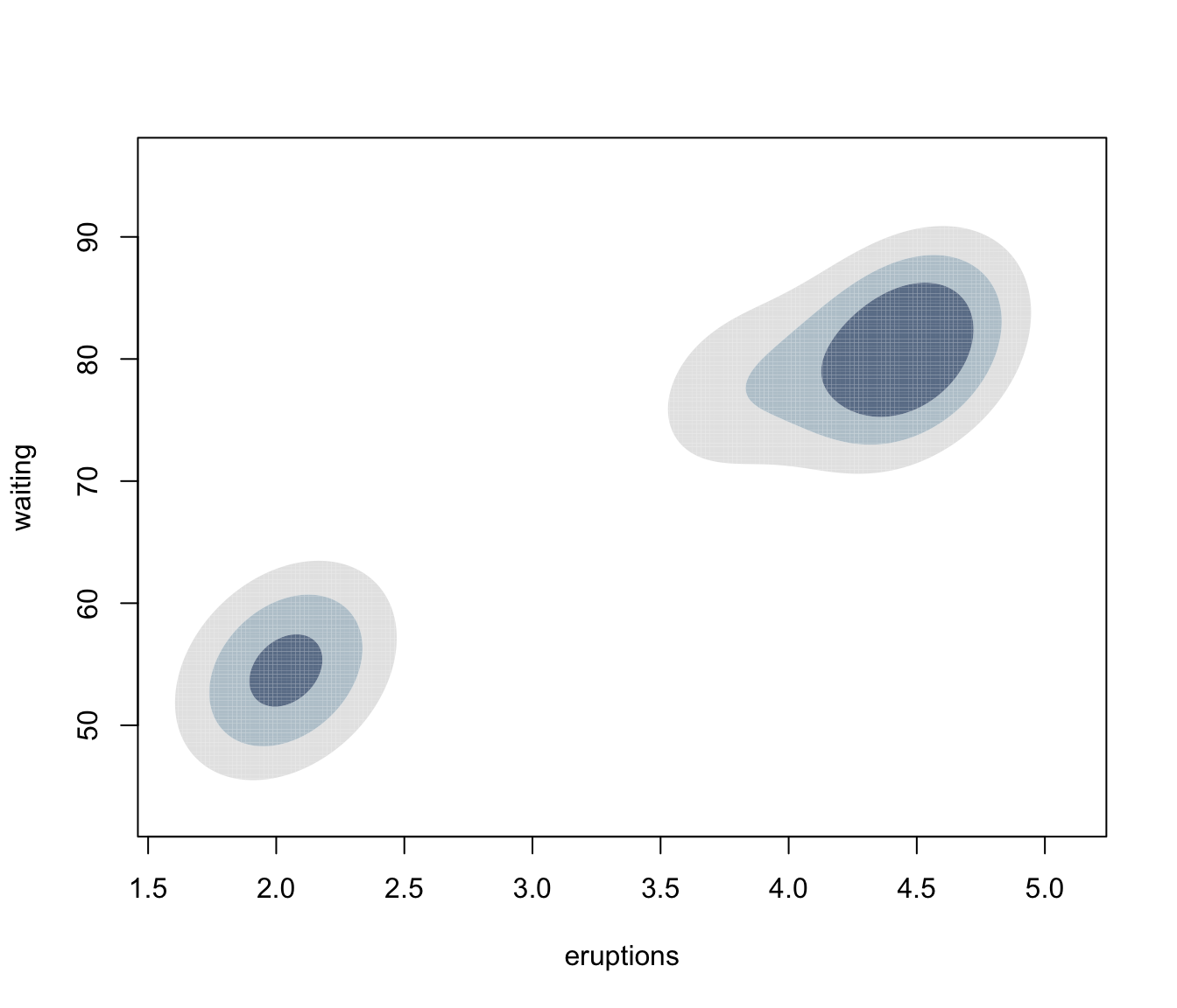
 plot(dens, what = "density", type = "hdr", data = faithful)
 plot(dens, what = "density", type = "persp")
 dens <- densityMclust(iris[,1:4], plot = FALSE)
summary(dens, parameters = TRUE)
#> -------------------------------------------------------
#> Density estimation via Gaussian finite mixture modeling
#> -------------------------------------------------------
#>
#> Mclust VEV (ellipsoidal, equal shape) model with 2 components:
#>
#> log-likelihood n df BIC ICL
#> -215.726 150 26 -561.7285 -561.7289
#>
#> Mixing probabilities:
#> 1 2
#> 0.3333319 0.6666681
#>
#> Means:
#> [,1] [,2]
#> Sepal.Length 5.0060022 6.261996
#> Sepal.Width 3.4280049 2.871999
#> Petal.Length 1.4620007 4.905992
#> Petal.Width 0.2459998 1.675997
#>
#> Variances:
#> [,,1]
#> Sepal.Length Sepal.Width Petal.Length Petal.Width
#> Sepal.Length 0.15065114 0.13080115 0.02084463 0.01309107
#> Sepal.Width 0.13080115 0.17604529 0.01603245 0.01221458
#> Petal.Length 0.02084463 0.01603245 0.02808260 0.00601568
#> Petal.Width 0.01309107 0.01221458 0.00601568 0.01042365
#> [,,2]
#> Sepal.Length Sepal.Width Petal.Length Petal.Width
#> Sepal.Length 0.4000438 0.10865444 0.3994018 0.14368256
#> Sepal.Width 0.1086544 0.10928077 0.1238904 0.07284384
#> Petal.Length 0.3994018 0.12389040 0.6109024 0.25738990
#> Petal.Width 0.1436826 0.07284384 0.2573899 0.16808182
plot(dens, what = "density", data = iris[,1:4],
col = "slategrey", drawlabels = FALSE, nlevels = 7)
dens <- densityMclust(iris[,1:4], plot = FALSE)
summary(dens, parameters = TRUE)
#> -------------------------------------------------------
#> Density estimation via Gaussian finite mixture modeling
#> -------------------------------------------------------
#>
#> Mclust VEV (ellipsoidal, equal shape) model with 2 components:
#>
#> log-likelihood n df BIC ICL
#> -215.726 150 26 -561.7285 -561.7289
#>
#> Mixing probabilities:
#> 1 2
#> 0.3333319 0.6666681
#>
#> Means:
#> [,1] [,2]
#> Sepal.Length 5.0060022 6.261996
#> Sepal.Width 3.4280049 2.871999
#> Petal.Length 1.4620007 4.905992
#> Petal.Width 0.2459998 1.675997
#>
#> Variances:
#> [,,1]
#> Sepal.Length Sepal.Width Petal.Length Petal.Width
#> Sepal.Length 0.15065114 0.13080115 0.02084463 0.01309107
#> Sepal.Width 0.13080115 0.17604529 0.01603245 0.01221458
#> Petal.Length 0.02084463 0.01603245 0.02808260 0.00601568
#> Petal.Width 0.01309107 0.01221458 0.00601568 0.01042365
#> [,,2]
#> Sepal.Length Sepal.Width Petal.Length Petal.Width
#> Sepal.Length 0.4000438 0.10865444 0.3994018 0.14368256
#> Sepal.Width 0.1086544 0.10928077 0.1238904 0.07284384
#> Petal.Length 0.3994018 0.12389040 0.6109024 0.25738990
#> Petal.Width 0.1436826 0.07284384 0.2573899 0.16808182
plot(dens, what = "density", data = iris[,1:4],
col = "slategrey", drawlabels = FALSE, nlevels = 7)
 plot(dens, what = "density", type = "hdr", data = iris[,1:4])
 plot(dens, what = "density", type = "persp", col = grey(0.9))
 # }
# }