Modeling log-returns distribution via Gaussian Mixture Models

Gaussian mixtures for modeling the distribution of financial log-returns.

Usage

GMMlogreturn(y, ...)

# S3 method for class 'GMMlogreturn'
summary(object, ...)

Arguments

y: A numeric vector providing the log-returns of a financial stock.
...: Further arguments passed to mclust::densityMclust(). For a full description of available arguments see the corresponding help page.
object: An object of class 'GMMlogreturn'.

Value

Returns an object of class 'GMMlogreturn'.

Details

Let $P_t$ be the price of a financial stock for the current time frame (day for instance), and $P_{t-1}$ the price of the previous time frame. The log-return at time $t$ is defined as: $$ y_t = \log( \frac{P_t}{P_{t-1}} ) $$ By default, a univariate heteroscedastic GMM using Bayesian regularization (as described in mclust::priorControl()) is fitted to the observed log-returns. The number of mixture components is automatically selected by BIC, unless specified with the optional G argument.

References

Scrucca L. (2024) Entropy-based volatility analysis of financial log-returns using Gaussian mixture models. Entropy, 26(11), 907. doi:10.3390/e26110907

Author

Luca Scrucca

Examples

data(gold)
head(gold)
#>         date   log.returns
#> 1 2023-01-03  0.0109308628
#> 2 2023-01-04  0.0070955464
#> 3 2023-01-05 -0.0097625244
#> 4 2023-01-06  0.0158964701
#> 5 2023-01-09  0.0045492333
#> 6 2023-01-10 -0.0005875467
mod = GMMlogreturn(gold$log.returns)
summary(mod)
#> ── Log-returns density estimation via Gaussian finite mixture modeling ─────────
#> Model: GMM(V,2)
#> Prior: defaultPrior()
#> 
#>  log-likelihood   n df    BIC Entropy
#>          852.46 250  5 1677.3 -3.4098
#> 
#> Mixture parameters:
#>      Prob       Mean     StDev
#> 1 0.52433 0.00029069 0.0045432
#> 2 0.47567 0.00073238 0.0107633
#> 
#> Marginal statistics:
#>        Mean     StDev Skewness Kurtosis      VaR       ES
#>  0.00050079 0.0081227 0.058714   4.5584 0.012877 0.017929
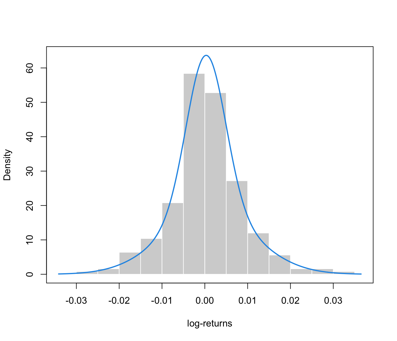
plot(mod, what = "density", data = gold$log.returns,
     xlab = "log-returns", col = 4, lwd = 2)