Subset selection for GMMDR directions based on BIC

Implements a subset selection method for selecting the relevant directions spanning the dimension reduction subspace for visualizing the clustering or classification structure obtained from a finite mixture of Gaussian densities.

Usage

MclustDRsubsel(object, G = 1:9,
                       modelNames = mclust.options("emModelNames"), 
                       ...,
                       bic.stop = 0, bic.cutoff = 0, 
                       mindir = 1, 
                       verbose = interactive())

Arguments

object

An object of class 'MclustDR' resulting from a call to MclustDR.

G

An integer vector specifying the numbers of mixture components or clusters.

modelNames

A vector of character strings indicating the models to be fitted. See mclustModelNames for a description of the available models.

...

Further arguments passed through Mclust or MclustDA.

bic.stop

A criterion to terminate the search. If maximal BIC difference is less than bic.stop then the algorithm stops.
Two tipical values are:

`0`:	algorithm stops when the BIC difference becomes negative (default);
`-Inf`:	algorithm continues until all directions have been selected.

bic.cutoff

A value specifying how to select simplest ``best'' model within bic.cutoff from the maximum value achieved. Setting this to 0 (default) simply select the model with the largest BIC difference.

mindir

An integer value specifying the minimum number of directions to be estimated.

verbose

A logical or integer value specifying if and how much detailed information should be reported during the iterations of the algorithm.
Possible values are:

`0` or `FALSE`:	no trace info is shown;
`1` or `TRUE`:	a trace info is shown at each step of the search;
`2`:	a more detailed trace info is is shown.

Details

The GMMDR method aims at reducing the dimensionality by identifying a set of linear combinations, ordered by importance as quantified by the associated eigenvalues, of the original features which capture most of the clustering or classification structure contained in the data. This is implemented in MclustDR.

The MclustDRsubsel function implements the greedy forward search algorithm discussed in Scrucca (2010) to prune the set of all GMMDR directions. The criterion used to select the relevant directions is based on the BIC difference between a clustering model and a model in which the feature proposal has no clustering relevance. The steps are the following:

1. Select the first feature to be the one which maximizes the BIC difference between the best clustering model and the model which assumes no clustering, i.e. a single component.

2. Select the next feature amongst those not previously included, to be the one which maximizes the BIC difference.

3. Iterate the previous step until all the BIC differences for the inclusion of a feature become less than bic.stop.

At each step, the search over the model space is performed with respect to the model parametrisation and the number of clusters.

Value

An object of class 'MclustDRsubsel' which inherits from 'MclustDR', so it has the same components of the latter plus the following:

basisx: The basis of the estimated dimension reduction subspace expressed in terms of the original variables.
std.basisx: The basis of the estimated dimension reduction subspace expressed in terms of the original variables standardized to have unit standard deviation.

References

Scrucca, L. (2010) Dimension reduction for model-based clustering. Statistics and Computing, 20(4), pp. 471-484.

Scrucca, L. (2014) Graphical Tools for Model-based Mixture Discriminant Analysis. Advances in Data Analysis and Classification, 8(2), pp. 147-165

Author

Luca Scrucca

Examples

# \donttest{
# clustering
data(crabs, package = "MASS")
x <- crabs[,4:8]
class <- paste(crabs$sp, crabs$sex, sep = "|")
mod <- Mclust(x)
table(class, mod$classification)
#>      
#> class  1  2  3  4
#>   B|F 49  0  0  1
#>   B|M 11  0 39  0
#>   O|F  0  5  0 45
#>   O|M  0 50  0  0
dr <- MclustDR(mod)
summary(dr)
#> ----------------------------------------------------------------- 
#> Dimension reduction for model-based clustering and classification 
#> ----------------------------------------------------------------- 
#> 
#> Mixture model type: Mclust (EEV, 4) 
#>         
#> Clusters  n
#>        1 60
#>        2 55
#>        3 39
#>        4 46
#> 
#> Estimated basis vectors: 
#>         Dir1     Dir2     Dir3
#> FL -0.598015 -0.10316 -0.68314
#> RW -0.327540 -0.67796  0.15897
#> CL  0.002013  0.52296  0.17400
#> CW  0.538877 -0.36100 -0.24560
#> BD -0.494675  0.35484  0.64610
#> 
#>                Dir1    Dir2       Dir3
#> Eigenvalues  1.5907  1.0782   0.099104
#> Cum. %      57.4678 96.4196 100.000000
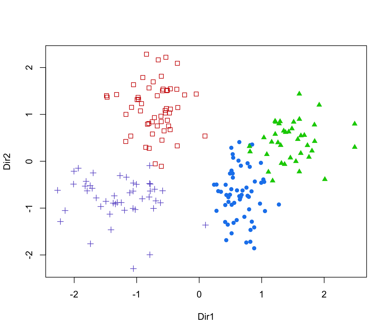
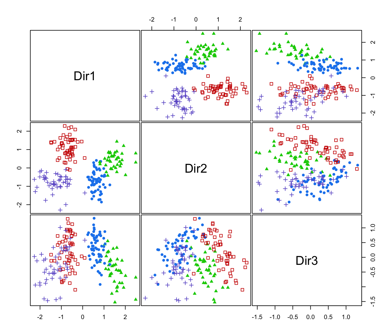
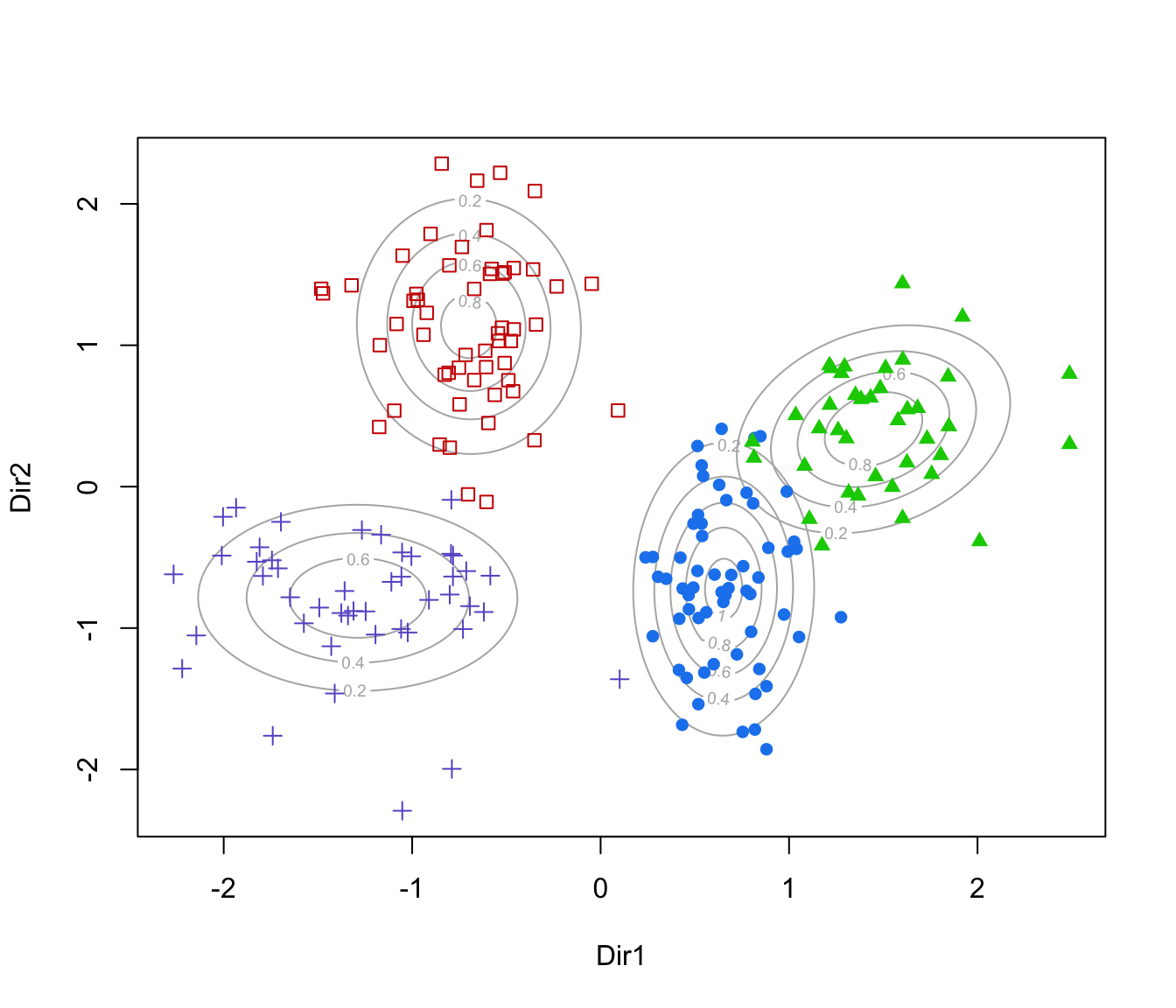
plot(dr)







drs <- MclustDRsubsel(dr)
summary(drs)
#> ----------------------------------------------------------------- 
#> Dimension reduction for model-based clustering and classification 
#> ----------------------------------------------------------------- 
#> 
#> Mixture model type: Mclust (EVE, 5) 
#>         
#> Clusters  n
#>        1 64
#>        2 36
#>        3 29
#>        4 41
#>        5 30
#> 
#> Estimated basis vectors: 
#>         Dir1       Dir2      Dir3
#> FL  0.659021 -0.1712004 -0.634547
#> RW  0.230063  0.8425324  0.027738
#> CL  0.037967 -0.4701147  0.254548
#> CW -0.548500  0.1994410 -0.299751
#> BD  0.458768  0.0067046  0.664783
#> 
#>                Dir1     Dir2      Dir3
#> Eigenvalues  1.7179  0.99776   0.20408
#> Cum. %      58.8367 93.01017 100.00000
table(class, drs$classification)
#>      
#> class  1  2  3  4  5
#>   B|F 50  0  0  0  0
#>   B|M 14 36  0  0  0
#>   O|F  0  0 19  1 30
#>   O|M  0  0 10 40  0
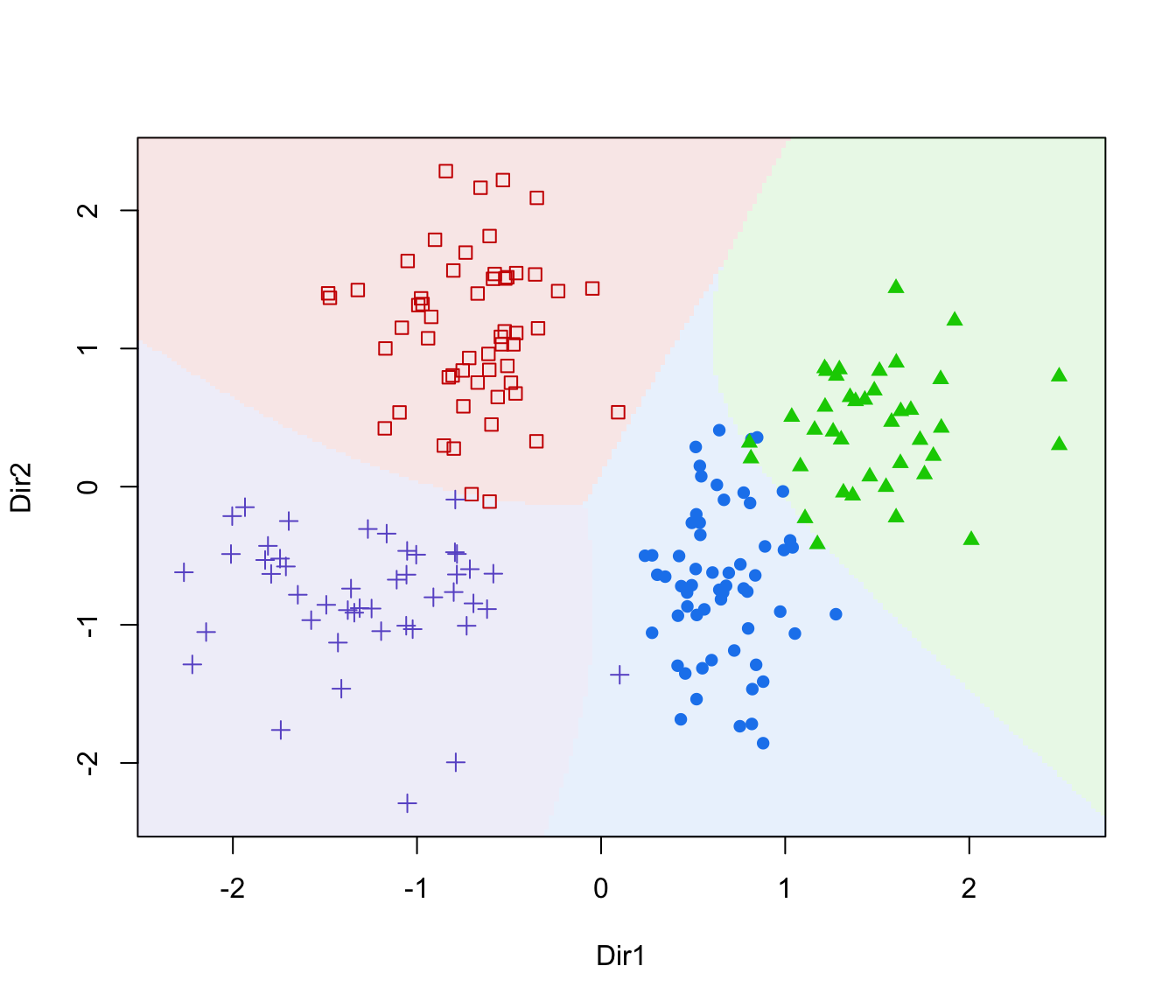
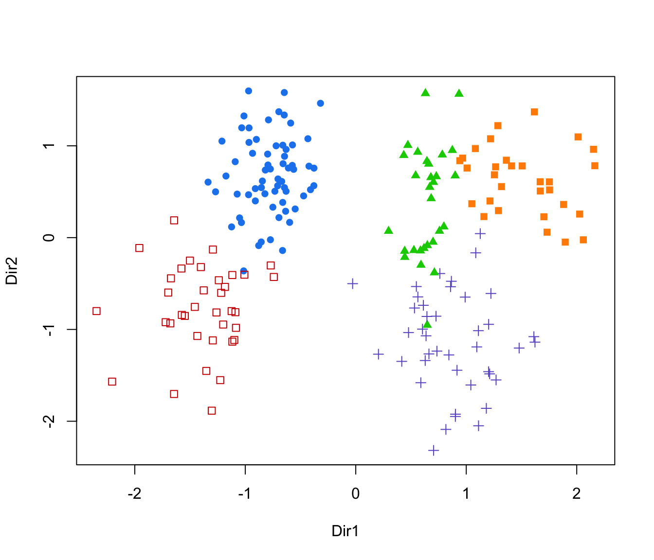
plot(drs, what = "scatterplot")

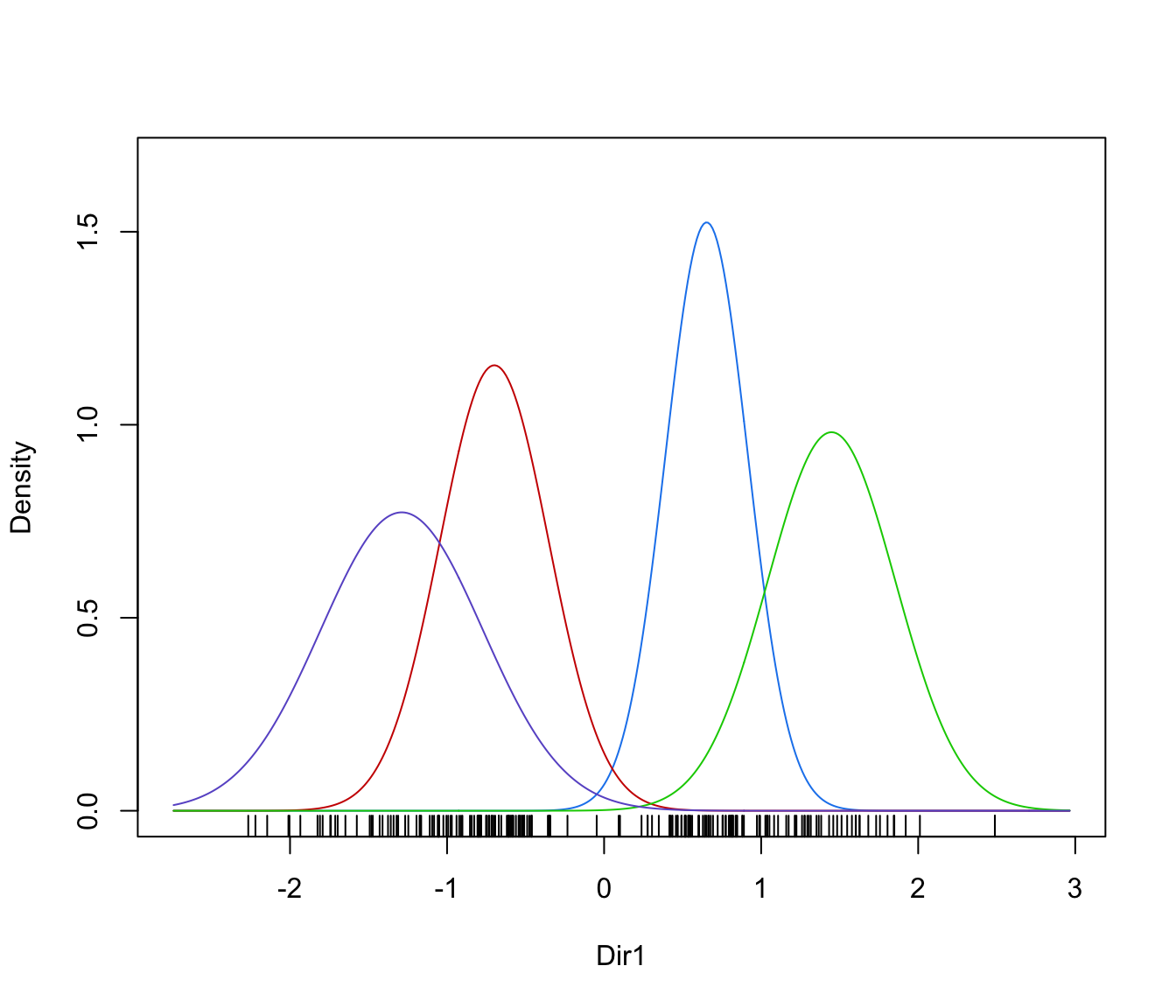
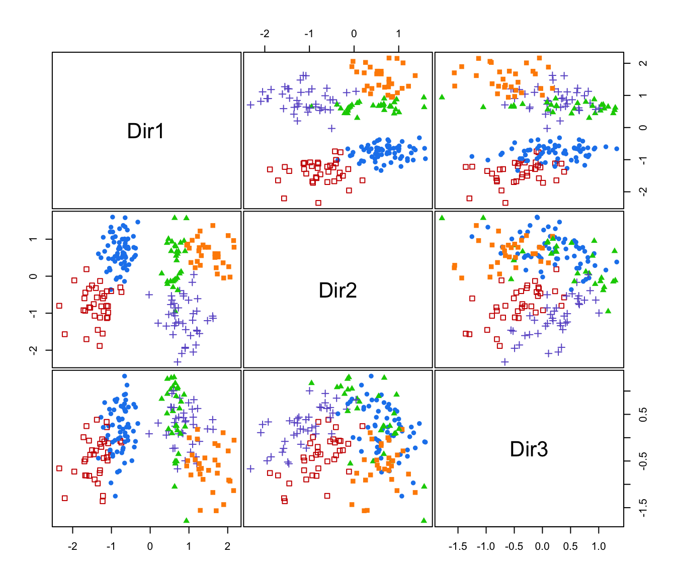
plot(drs, what = "pairs")

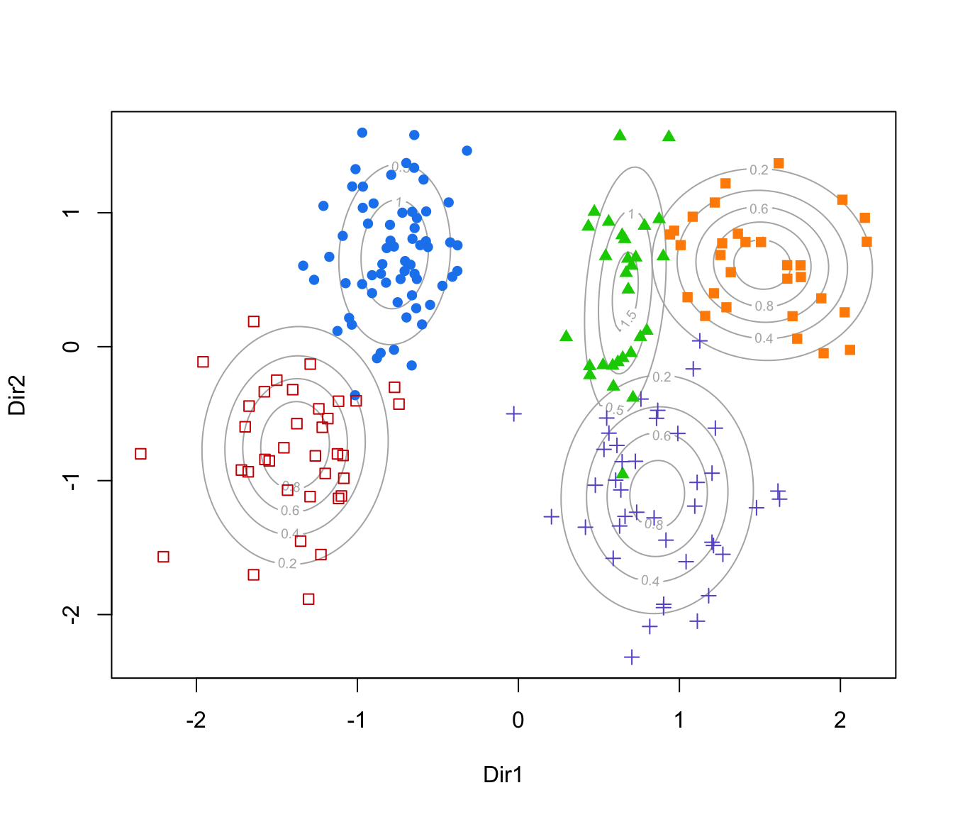
plot(drs, what = "contour")

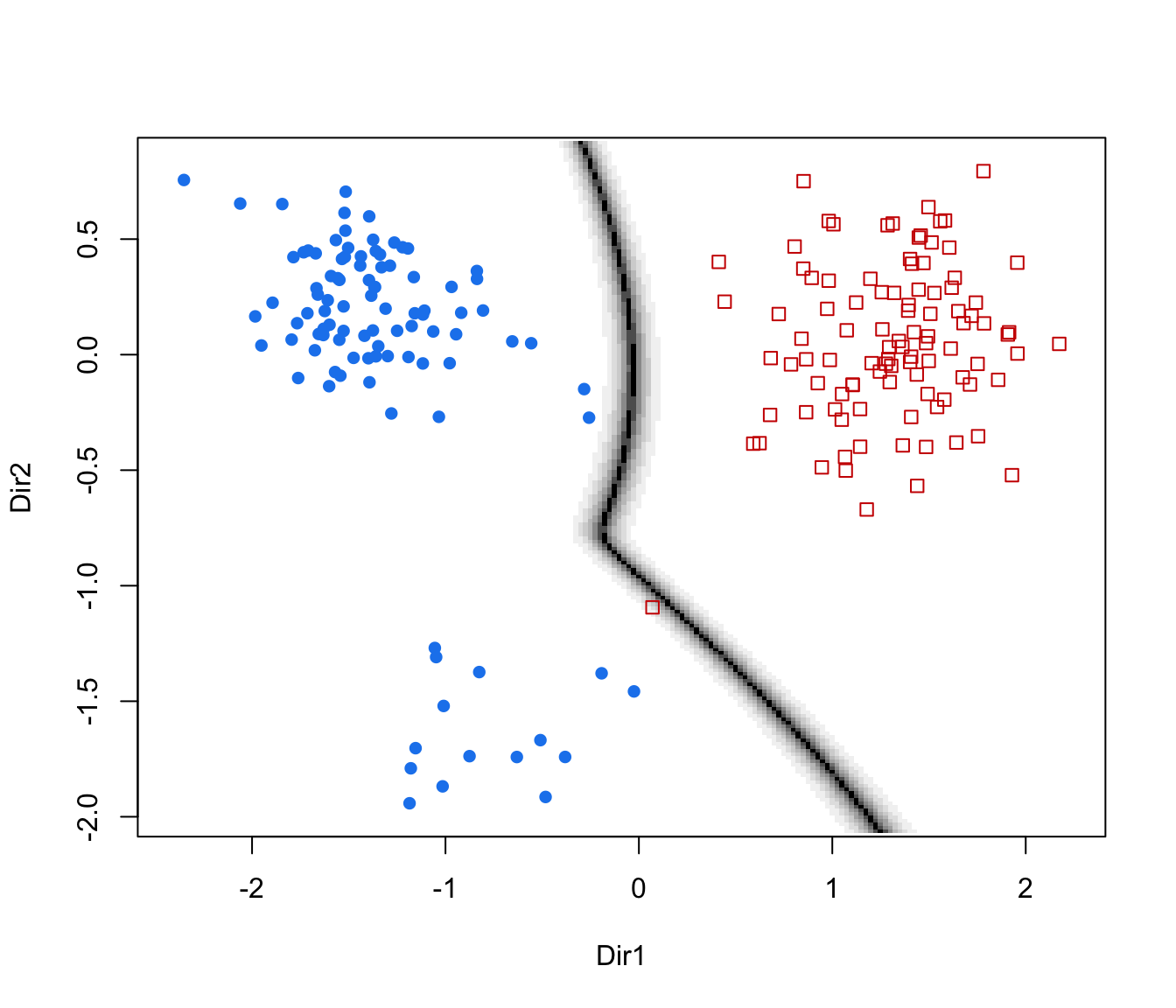
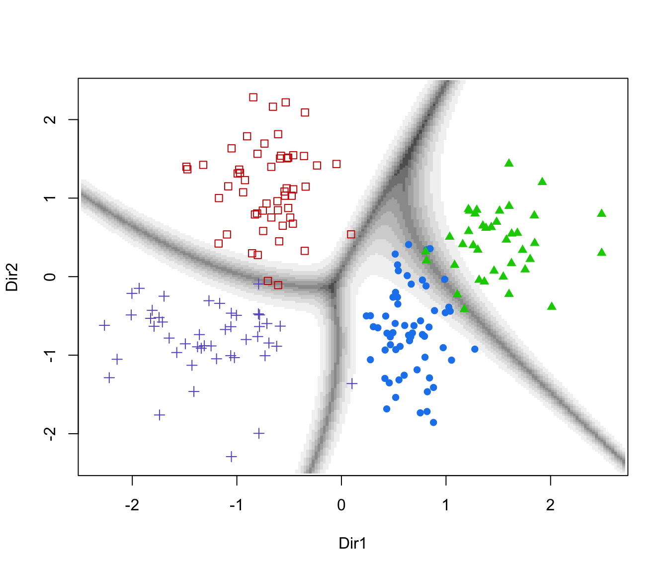
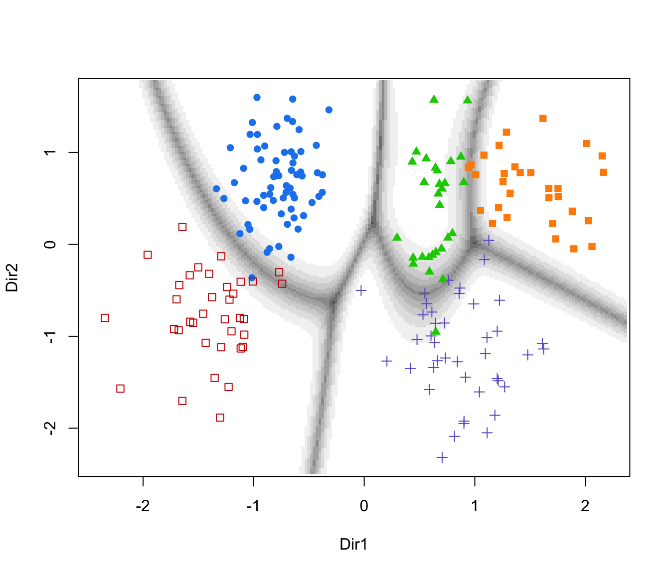
plot(drs, what = "boundaries")

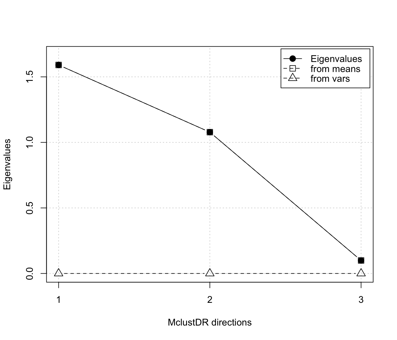
plot(drs, what = "evalues")


# classification
data(banknote)
da <- MclustDA(banknote[,2:7], banknote$Status)
table(banknote$Status, predict(da)$class)
#>              
#>               counterfeit genuine
#>   counterfeit         100       0
#>   genuine               0     100
dr <- MclustDR(da)
summary(dr)
#> ----------------------------------------------------------------- 
#> Dimension reduction for model-based clustering and classification 
#> ----------------------------------------------------------------- 
#> 
#> Mixture model type: MclustDA 
#>              
#> Classes         n Model G
#>   counterfeit 100   EVE 2
#>   genuine     100   XXX 1
#> 
#> Estimated basis vectors: 
#>              Dir1     Dir2
#> Length   -0.07016 -0.25690
#> Left     -0.36888 -0.19963
#> Right     0.29525 -0.10111
#> Bottom    0.54683  0.46254
#> Top       0.55720  0.41370
#> Diagonal -0.40290  0.70628
#> 
#>                Dir1     Dir2
#> Eigenvalues  1.7188   1.0607
#> Cum. %      61.8373 100.0000
drs <- MclustDRsubsel(dr)
summary(drs)
#> ----------------------------------------------------------------- 
#> Dimension reduction for model-based clustering and classification 
#> ----------------------------------------------------------------- 
#> 
#> Mixture model type: MclustDA 
#>              
#> Classes         n Model G
#>   counterfeit 100   EEE 2
#>   genuine     100   XII 1
#> 
#> Estimated basis vectors: 
#>              Dir1     Dir2
#> Length    0.07016 -0.25690
#> Left      0.36888 -0.19963
#> Right    -0.29525 -0.10111
#> Bottom   -0.54683  0.46254
#> Top      -0.55720  0.41370
#> Diagonal  0.40290  0.70628
#> 
#>                Dir1     Dir2
#> Eigenvalues  1.7188   1.0607
#> Cum. %      61.8373 100.0000
table(banknote$Status, predict(drs)$class)
#>              
#>               counterfeit genuine
#>   counterfeit         100       0
#>   genuine               1      99
plot(drs, what = "scatterplot")

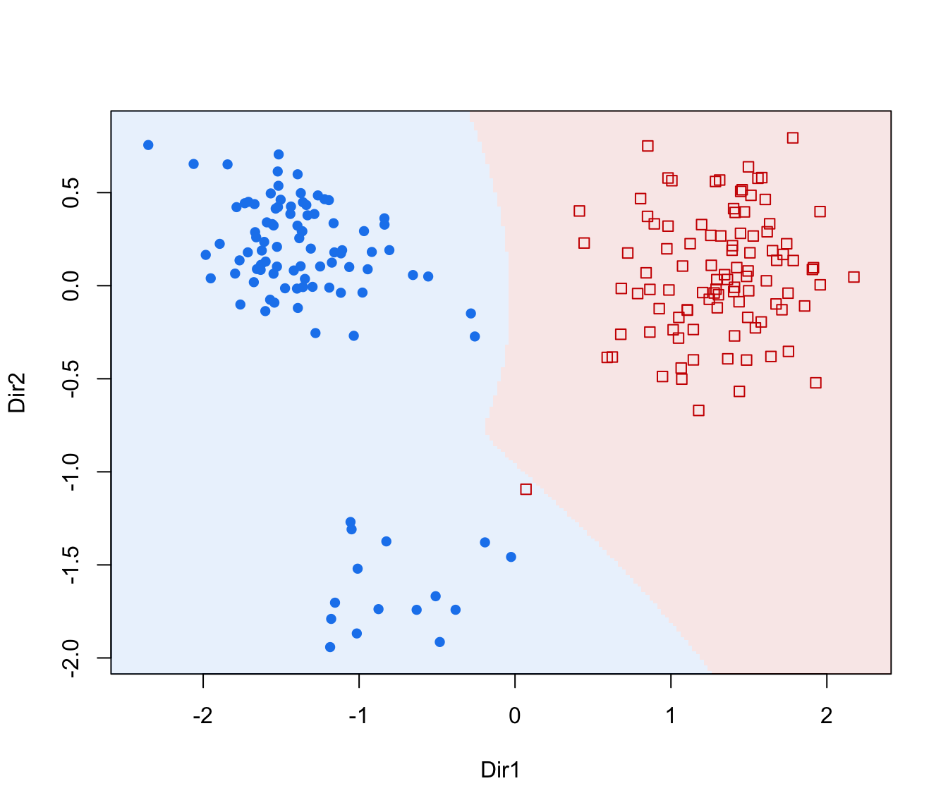
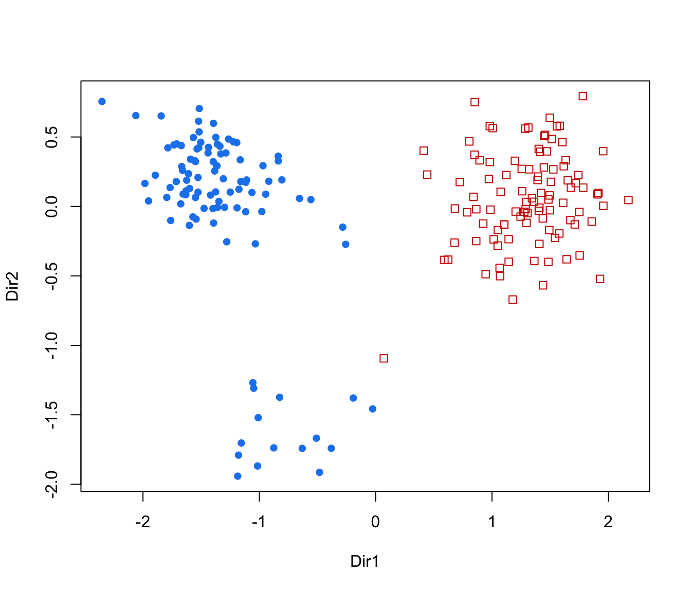plot(drs, what = "classification")

plot(drs, what = "boundaries")# }