Cumulative Distribution and Quantiles for a univariate Gaussian mixture distribution

Compute the cumulative density function (cdf) or quantiles from an estimated one-dimensional Gaussian mixture fitted using densityMclust.

Usage

cdfMclust(object, data, ngrid = 100, ...)
quantileMclust(object, p, ...)

Arguments

object: a densityMclust model object.
data: a numeric vector of evaluation points.
ngrid: the number of points in a regular grid to be used as evaluation points if no data are provided.
p: a numeric vector of probabilities.
...: further arguments passed to or from other methods.

Details

The cdf is evaluated at points given by the optional argument data. If not provided, a regular grid of length ngrid for the evaluation points is used.

The quantiles are computed using bisection linear search algorithm.

Value

cdfMclust returns a list of x and y values providing, respectively, the evaluation points and the estimated cdf.

quantileMclust returns a vector of quantiles.

Author

Luca Scrucca

Examples

# \donttest{
x <- c(rnorm(100), rnorm(100, 3, 2))
dens <- densityMclust(x, plot = FALSE)
summary(dens, parameters = TRUE)
#> ------------------------------------------------------- 
#> Density estimation via Gaussian finite mixture modeling 
#> ------------------------------------------------------- 
#> 
#> Mclust V (univariate, unequal variance) model with 2 components: 
#> 
#>  log-likelihood   n df      BIC       ICL
#>       -425.5477 200  5 -877.587 -958.5984
#> 
#> Mixing probabilities:
#>         1         2 
#> 0.4534143 0.5465857 
#> 
#> Means:
#>             1             2 
#> -0.0008132628  2.6833837538 
#> 
#> Variances:
#>         1         2 
#> 0.8244077 5.1023880 
cdf <- cdfMclust(dens)
str(cdf)
#> List of 2
#>  $ x: num [1:100] -4.26 -4.12 -3.98 -3.84 -3.7 ...
#>  $ y: num [1:100] 0.000575 0.000709 0.000872 0.001069 0.001307 ...
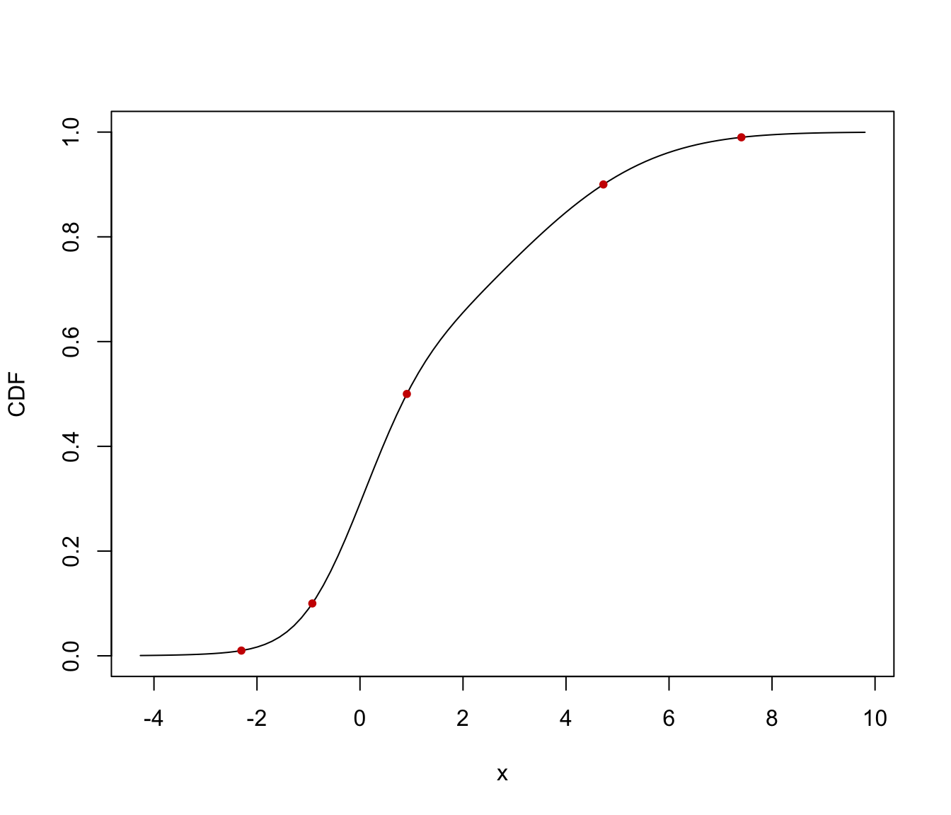
q <- quantileMclust(dens, p = c(0.01, 0.1, 0.5, 0.9, 0.99))
cbind(quantile = q, cdf = cdfMclust(dens, q)$y)
#>        quantile  cdf
#> [1,] -2.3030449 0.01
#> [2,] -0.9257016 0.10
#> [3,]  0.9100315 0.50
#> [4,]  4.7257546 0.90
#> [5,]  7.4050526 0.99
plot(cdf, type = "l", xlab = "x", ylab = "CDF")
points(q, cdfMclust(dens, q)$y, pch = 20, col = "red3")


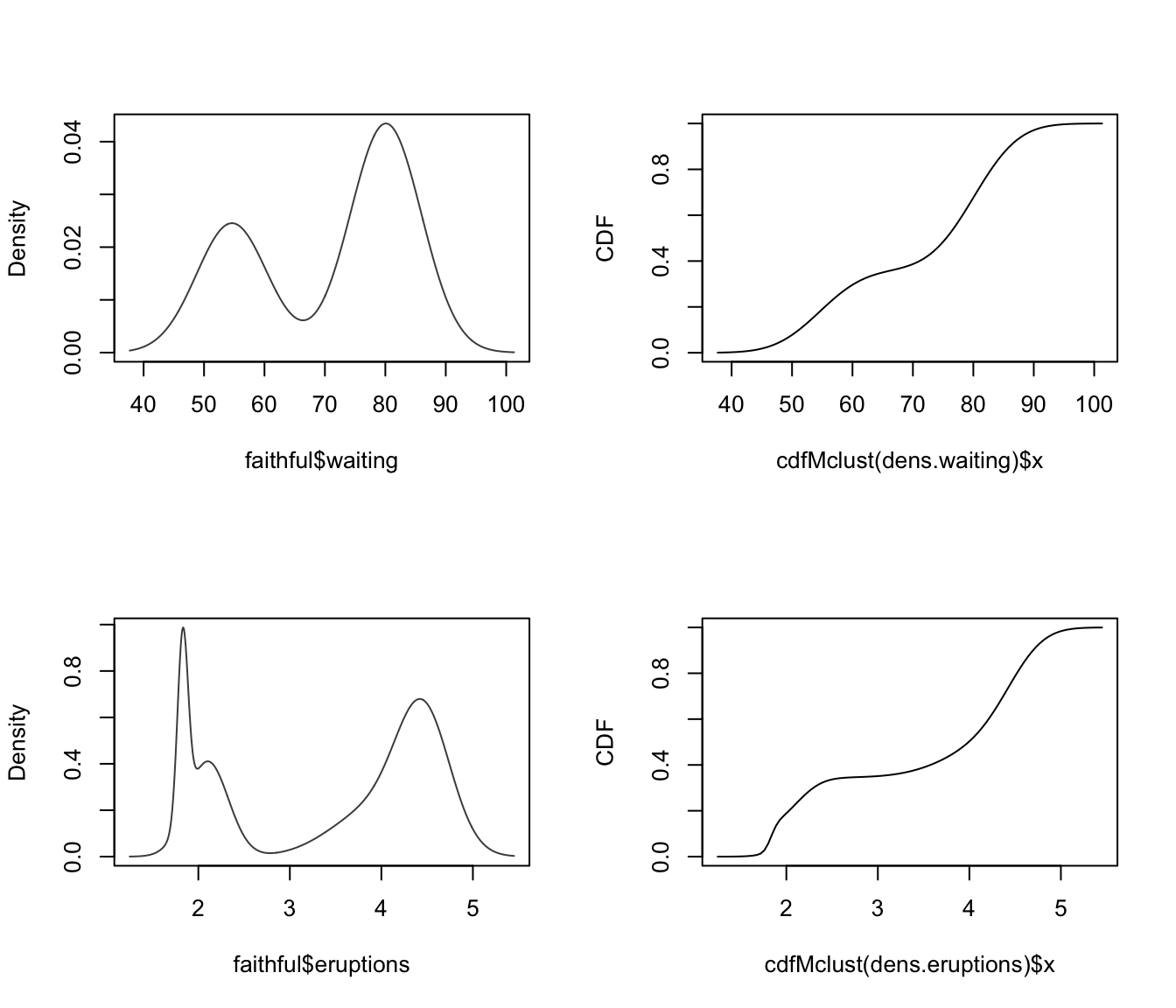
par(mfrow = c(2,2))
dens.waiting <- densityMclust(faithful$waiting)
plot(cdfMclust(dens.waiting), type = "l", 
     xlab = dens.waiting$varname, ylab = "CDF")
dens.eruptions <- densityMclust(faithful$eruptions)
plot(cdfMclust(dens.eruptions), type = "l", 
     xlab = dens.eruptions$varname, ylab = "CDF")

par(mfrow = c(1,1))
# }