Diagnostic plots for mclustDensity estimation — densityMclust.diagnostic • mclust

Diagnostic plots for density estimation. Only available for the one-dimensional case.

Usage

densityMclust.diagnostic(object, type = c("cdf", "qq"), 
                         col = c("black", "black"), 
                         lwd = c(2,1), lty = c(1,1), 
                         legend = TRUE, grid = TRUE, 
                         ...)

Arguments

object

An object of class 'mclustDensity' obtained from a call to densityMclust function.

type

The type of graph requested:

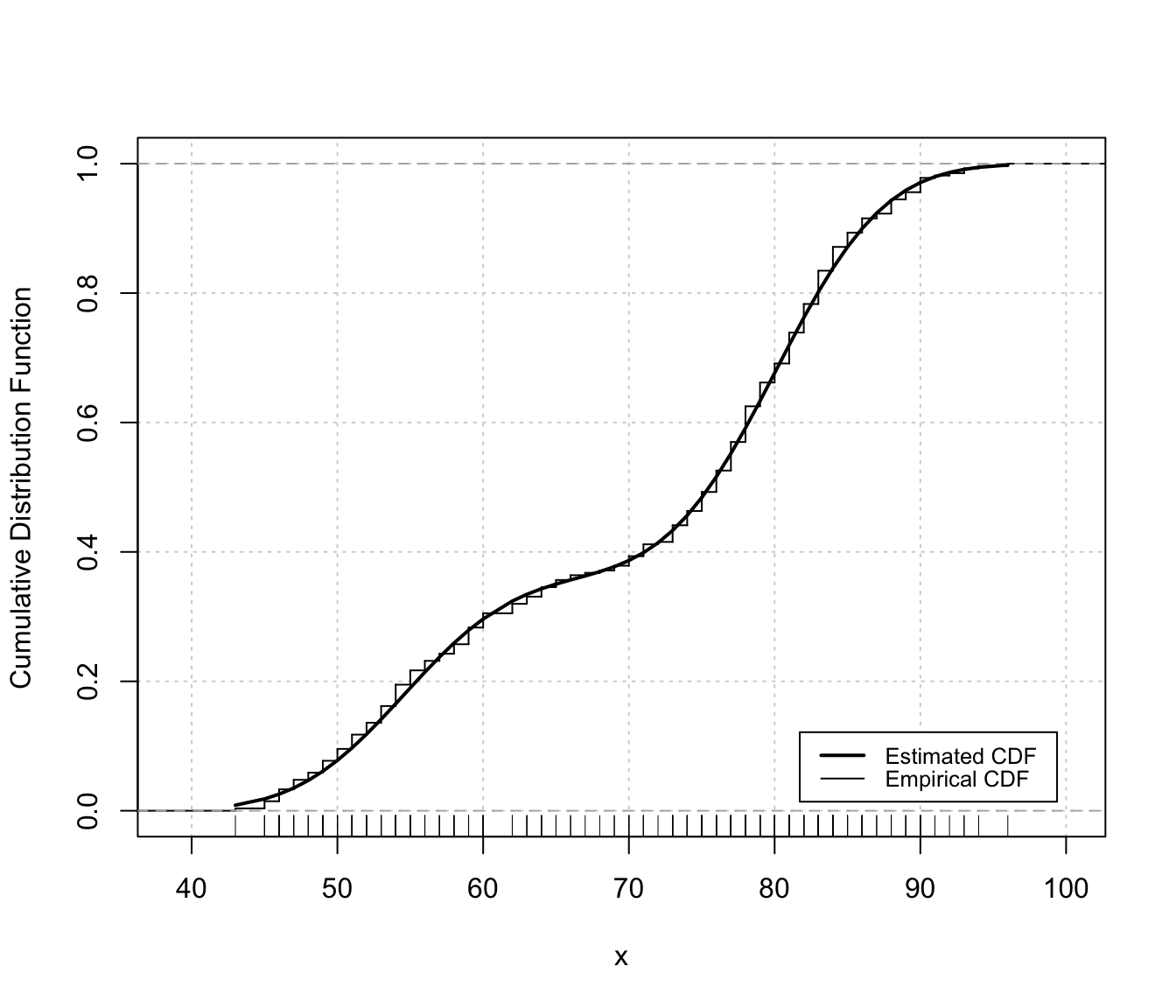
"cdf" =: a plot of the estimated CDF versus the empirical distribution function.
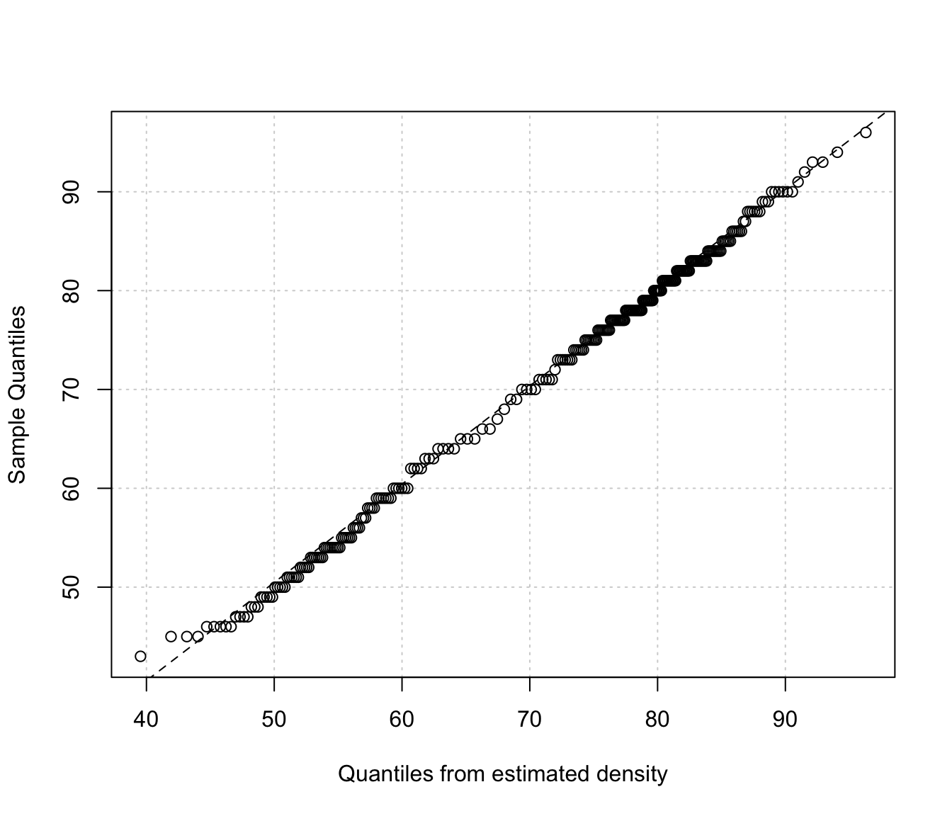
"qq" =: a Q-Q plot of sample quantiles versus the quantiles obtained from the inverse of the estimated cdf.

col

A pair of values for the color to be used for plotting, respectively, the estimated CDF and the empirical cdf.

lwd

A pair of values for the line width to be used for plotting, respectively, the estimated CDF and the empirical cdf.

lty

A pair of values for the line type to be used for plotting, respectively, the estimated CDF and the empirical cdf.

legend

A logical indicating if a legend must be added to the plot of fitted CDF vs the empirical CDF.

grid

A logical indicating if a grid should be added to the plot.

...

Additional arguments.

Details

The two diagnostic plots for density estimation in the one-dimensional case are discussed in Loader (1999, pp- 87-90).

References

Loader C. (1999), Local Regression and Likelihood. New York, Springer.

Scrucca L., Fraley C., Murphy T. B. and Raftery A. E. (2023) Model-Based Clustering, Classification, and Density Estimation Using mclust in R. Chapman & Hall/CRC, ISBN: 978-1032234953, https://mclust-org.github.io/book/

Author

Luca Scrucca

Examples

# \donttest{
x <- faithful$waiting
dens <- densityMclust(x, plot = FALSE)
plot(dens, x, what = "diagnostic")


# or
densityMclust.diagnostic(dens, type = "cdf")

densityMclust.diagnostic(dens, type = "qq")

# }

Diagnostic plots for `mclustDensity` estimation