Gaussian Mixture Modelling for Model-Based Clustering, Classification, and Density Estimation
mclust-package.RdGaussian finite mixture models estimated via EM algorithm for model-based clustering, classification, and density estimation, including Bayesian regularization and dimension reduction.
Details
For a quick introduction to mclust see the vignette A quick tour of mclust.
See also:
Mclustfor clustering;MclustDAfor supervised classification;MclustSSCfor semi-supervised classification;densityMclustfor density estimation.
Author
Chris Fraley, Adrian Raftery and Luca Scrucca.
Maintainer: Luca Scrucca luca.scrucca@unipg.it
References
Scrucca L., Fraley C., Murphy T. B. and Raftery A. E. (2023) Model-Based Clustering, Classification, and Density Estimation Using mclust in R. Chapman & Hall/CRC, ISBN: 978-1032234953, https://mclust-org.github.io/book/
Scrucca L., Fop M., Murphy T. B. and Raftery A. E. (2016) mclust 5: clustering, classification and density estimation using Gaussian finite mixture models, The R Journal, 8/1, pp. 289-317.
Fraley C. and Raftery A. E. (2002) Model-based clustering, discriminant analysis and density estimation, Journal of the American Statistical Association, 97/458, pp. 611-631.
Examples
# \donttest{
# Clustering
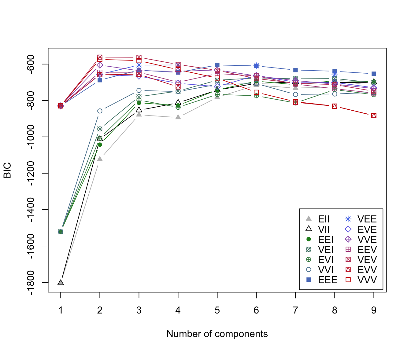
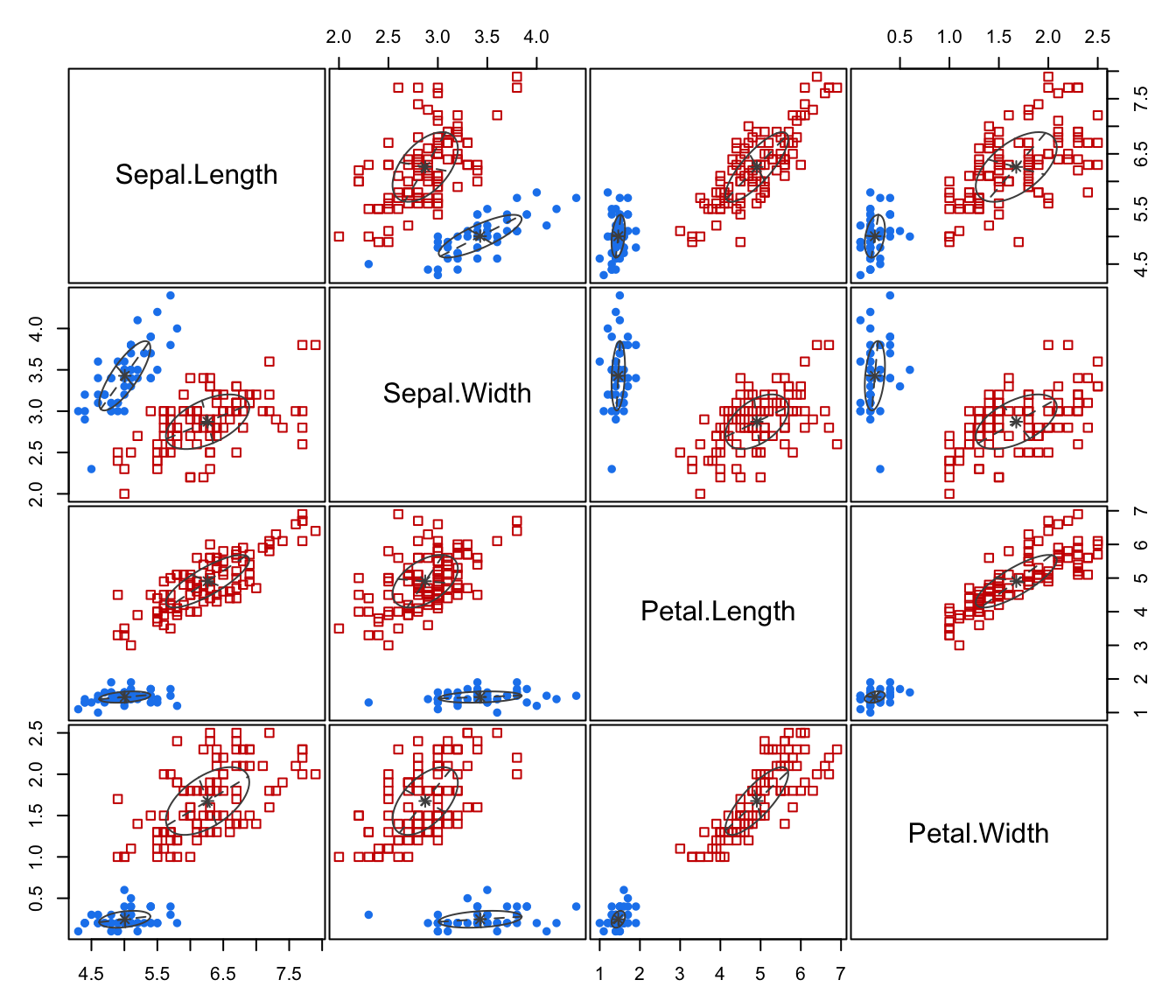
mod1 <- Mclust(iris[,1:4])
summary(mod1)
#> ----------------------------------------------------
#> Gaussian finite mixture model fitted by EM algorithm
#> ----------------------------------------------------
#>
#> Mclust VEV (ellipsoidal, equal shape) model with 2 components:
#>
#> log-likelihood n df BIC ICL
#> -215.726 150 26 -561.7285 -561.7289
#>
#> Clustering table:
#> 1 2
#> 50 100
plot(mod1, what = c("BIC", "classification"))
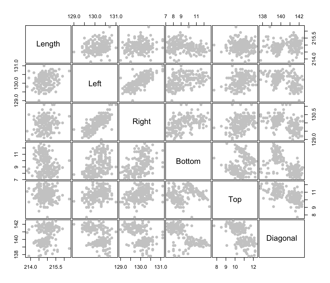
 # Classification
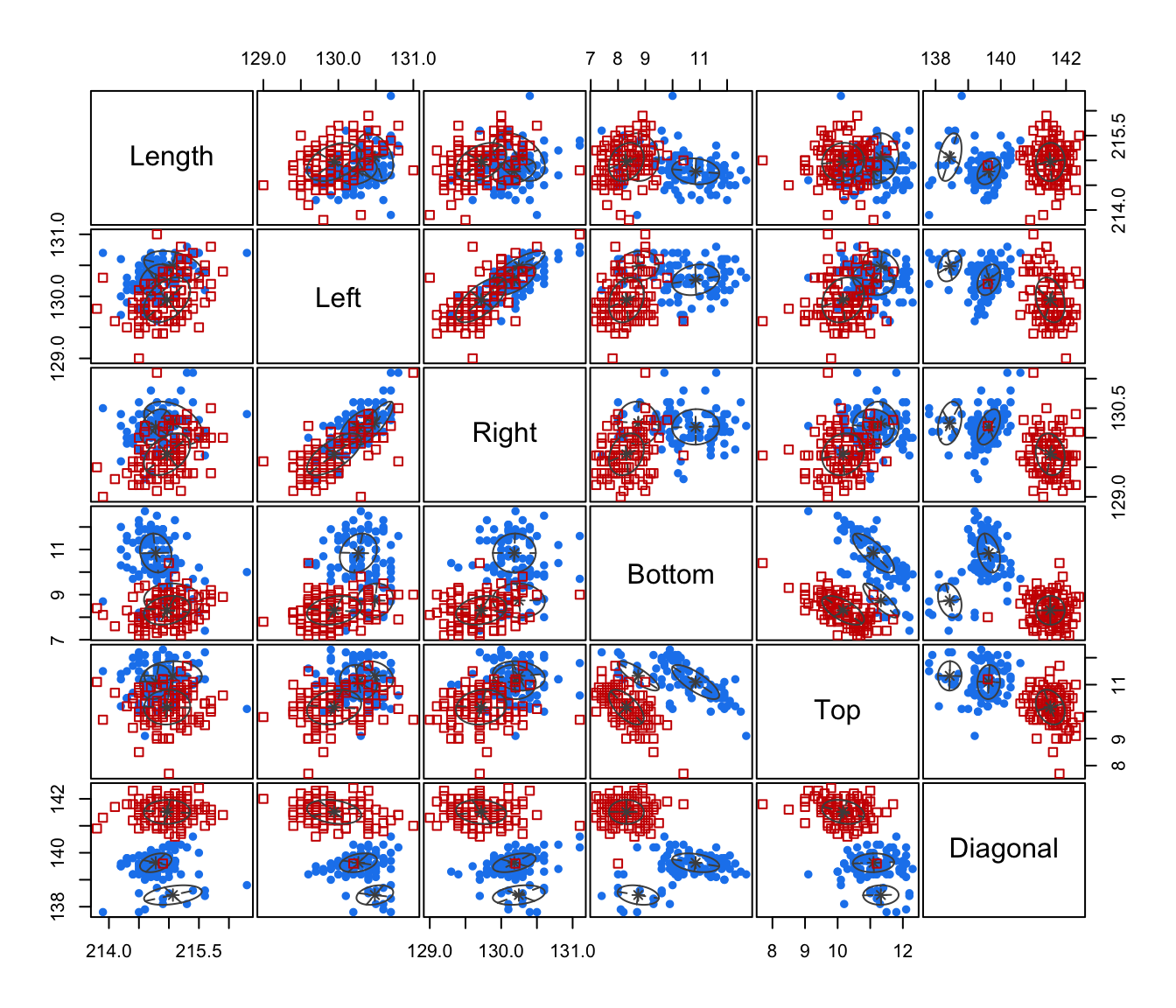
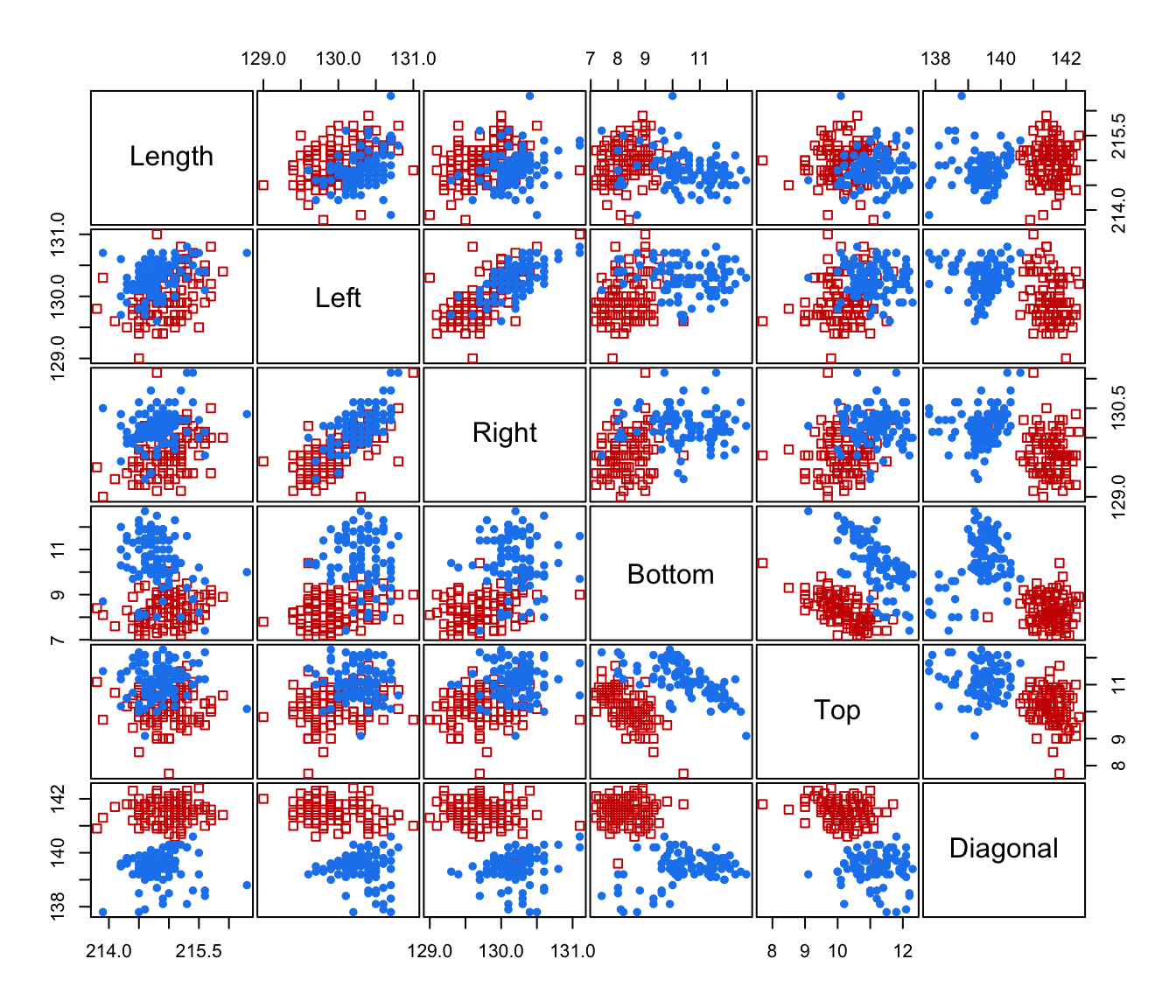
data(banknote)
mod2 <- MclustDA(banknote[,2:7], banknote$Status)
summary(mod2)
#> ------------------------------------------------
#> Gaussian finite mixture model for classification
#> ------------------------------------------------
#>
#> MclustDA
#> ------------------------------------------------
#> log-likelihood n df BIC
#> -646.0801 200 67 -1647.147
#>
#> Classes n % Model G
#> counterfeit 100 50 EVE 2
#> genuine 100 50 XXX 1
#>
#> Training confusion matrix
#> ------------------------------------------------
#> Predicted
#> Classes counterfeit genuine
#> counterfeit 100 0
#> genuine 0 100
#>
#> Classification error = 0.0000
#> Brier score = 0.0000
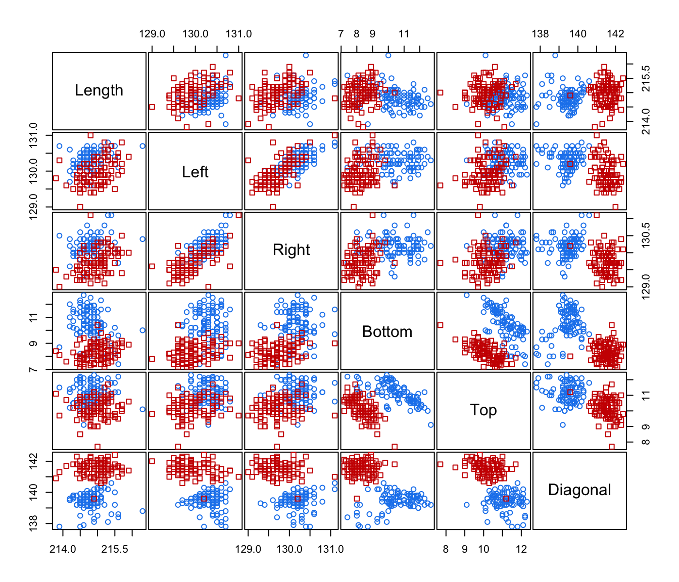
plot(mod2)
# Classification
data(banknote)
mod2 <- MclustDA(banknote[,2:7], banknote$Status)
summary(mod2)
#> ------------------------------------------------
#> Gaussian finite mixture model for classification
#> ------------------------------------------------
#>
#> MclustDA
#> ------------------------------------------------
#> log-likelihood n df BIC
#> -646.0801 200 67 -1647.147
#>
#> Classes n % Model G
#> counterfeit 100 50 EVE 2
#> genuine 100 50 XXX 1
#>
#> Training confusion matrix
#> ------------------------------------------------
#> Predicted
#> Classes counterfeit genuine
#> counterfeit 100 0
#> genuine 0 100
#>
#> Classification error = 0.0000
#> Brier score = 0.0000
plot(mod2)
 # Density estimation
mod3 <- densityMclust(faithful$waiting)
# Density estimation
mod3 <- densityMclust(faithful$waiting)
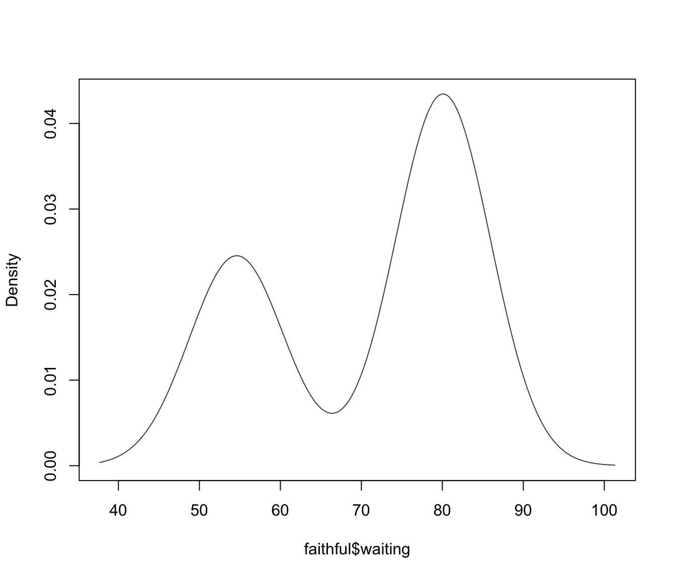 summary(mod3)
#> -------------------------------------------------------
#> Density estimation via Gaussian finite mixture modeling
#> -------------------------------------------------------
#>
#> Mclust E (univariate, equal variance) model with 2 components:
#>
#> log-likelihood n df BIC ICL
#> -1034.002 272 4 -2090.427 -2099.576
# }
summary(mod3)
#> -------------------------------------------------------
#> Density estimation via Gaussian finite mixture modeling
#> -------------------------------------------------------
#>
#> Mclust E (univariate, equal variance) model with 2 components:
#>
#> log-likelihood n df BIC ICL
#> -1034.002 272 4 -2090.427 -2099.576
# }