Plotting method for dimension reduction for model-based clustering and classification

Graphs data projected onto the estimated subspace for model-based clustering and classification.

Usage

# S3 method for MclustDR
plot(x, dimens, 
     what = c("scatterplot", "pairs", "contour", "classification",
              "boundaries", "density", "evalues"), 
     symbols, colors, col.contour = gray(0.7), col.sep = grey(0.4), 
     ngrid = 200, nlevels = 5, asp = NULL, ...)

Arguments

x

An object of class 'MclustDR' resulting from a call to MclustDR.

dimens

A vector of integers giving the dimensions of the desired coordinate projections for multivariate data.

what

The type of graph requested:

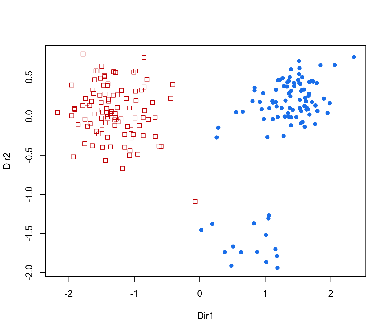
"scatterplot" =: a two-dimensional plot of data projected onto the first two directions specified by dimens and with data points marked according to the corresponding mixture component. By default, the first two directions are selected for plotting.
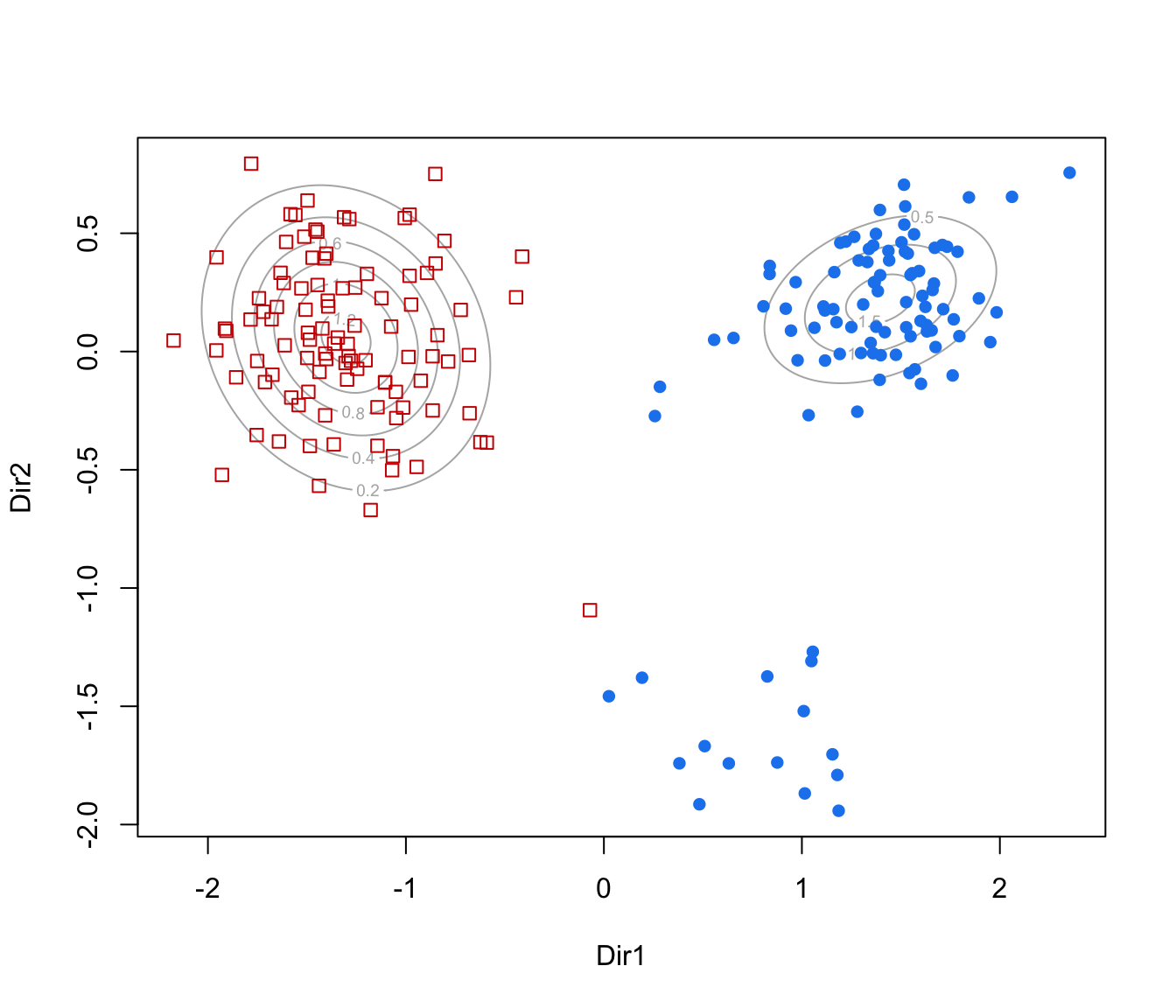
"pairs" =: a scatterplot matrix of data projected onto the estimated subspace and with data points marked according to the corresponding mixture component. By default, all the available directions are used, unless they have been specified by dimens.
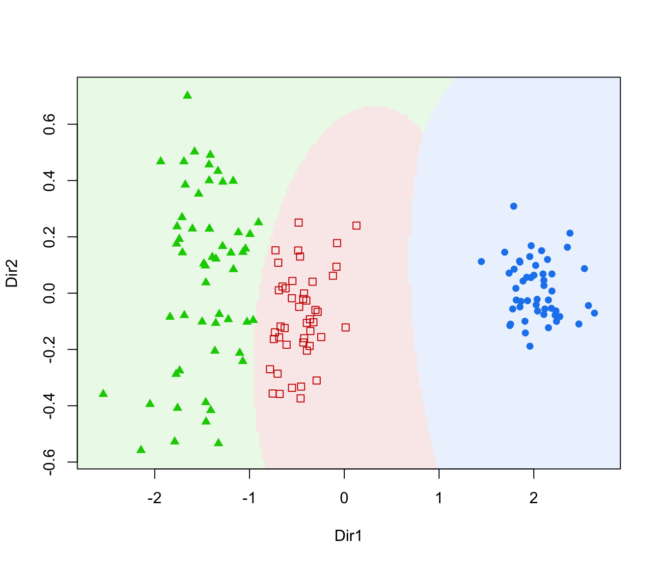
"contour" =: a two-dimensional plot of data projected onto the first two directions specified by dimens (by default, the first two directions) with density contours for classes or clusters and data points marked according to the corresponding mixture component.
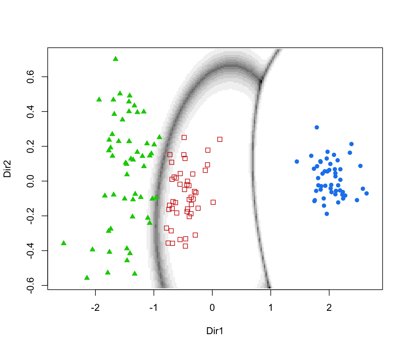
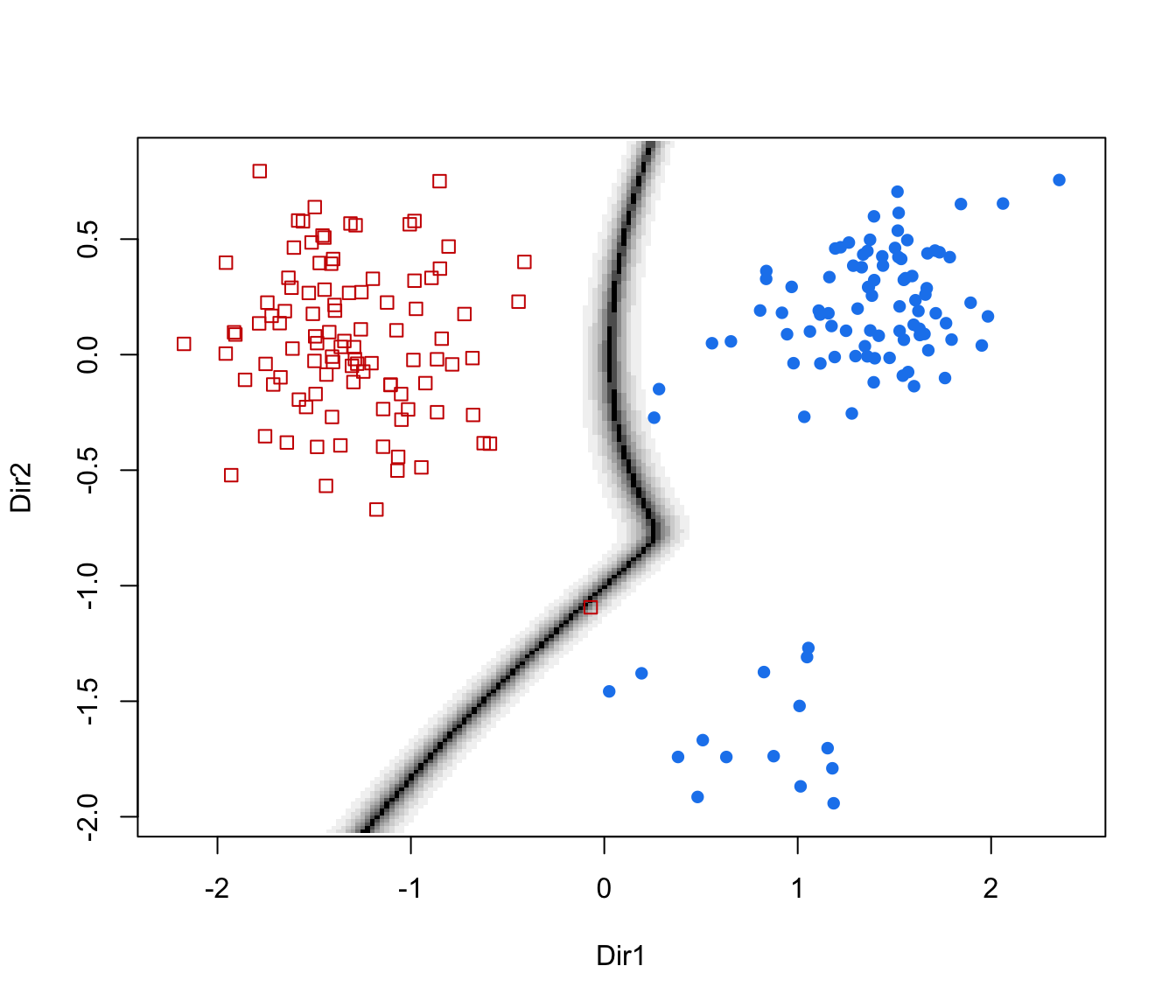
"classification" =: a two-dimensional plot of data projected onto the first two directions specified by dimens (by default, the first two directions) with classification region and data points marked according to the corresponding mixture component.
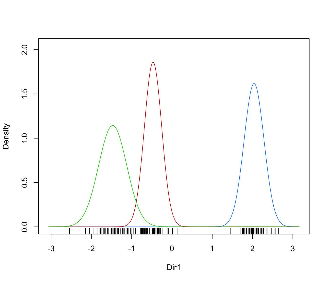
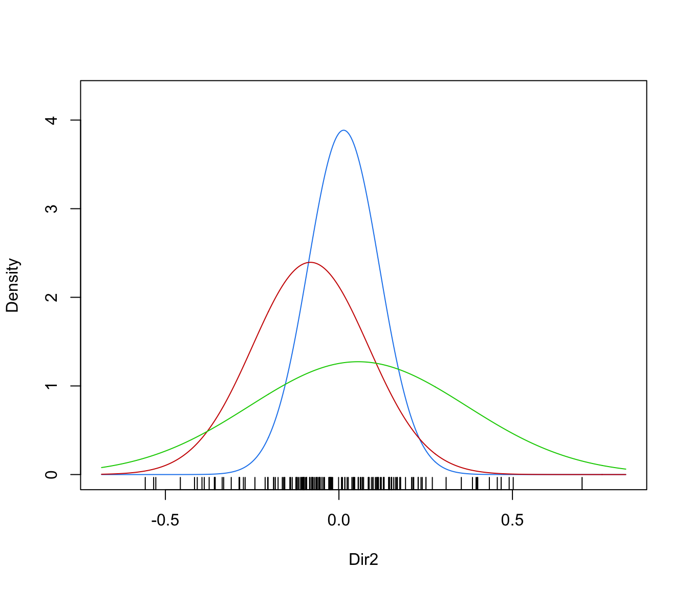
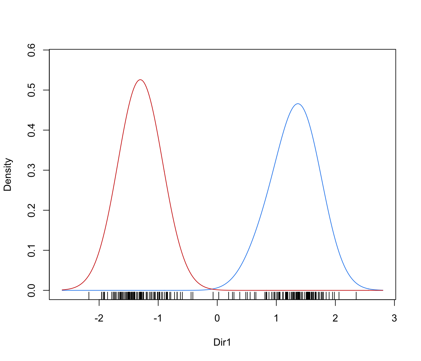
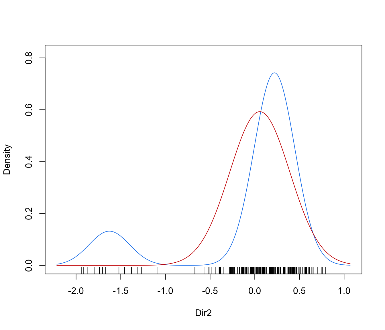
"boundaries" =: a two-dimensional plot of data projected onto the first two directions specified by dimens (by default, the first two directions) with uncertainty boundaries and data points marked according to the corresponding mixture component. The uncertainty is shown using a greyscale with darker regions indicating higher uncertainty.
"density" =: a one-dimensional plot of estimated density for the first direction specified by dimens (by default, the first one). A set of box-plots for each estimated cluster or known class are also shown at the bottom of the graph.

symbols

Either an integer or character vector assigning a plotting symbol to each unique mixture component. Elements in colors correspond to classes in order of appearance in the sequence of observations (the order used by the function factor). The default is given by mclust.options("classPlotSymbols").

colors

Either an integer or character vector assigning a color to each unique cluster or known class. Elements in colors correspond to classes in order of appearance in the sequence of observations (the order used by the function factor). The default is given by mclust.options("classPlotColors").

col.contour

The color of contours in case what = "contour".

col.sep

The color of classification boundaries in case what = "classification".

ngrid

An integer specifying the number of grid points to use in evaluating the classification regions.

nlevels

The number of levels to use in case what = "contour".

asp

For scatterplots the \(y/x\) aspect ratio, see plot.window.

...

further arguments passed to or from other methods.

References

Scrucca, L. (2010) Dimension reduction for model-based clustering. Statistics and Computing, 20(4), pp. 471-484.

Author

Luca Scrucca

Examples

# \donttest{
mod <- Mclust(iris[,1:4], G = 3)
dr <- MclustDR(mod, lambda = 0.5)
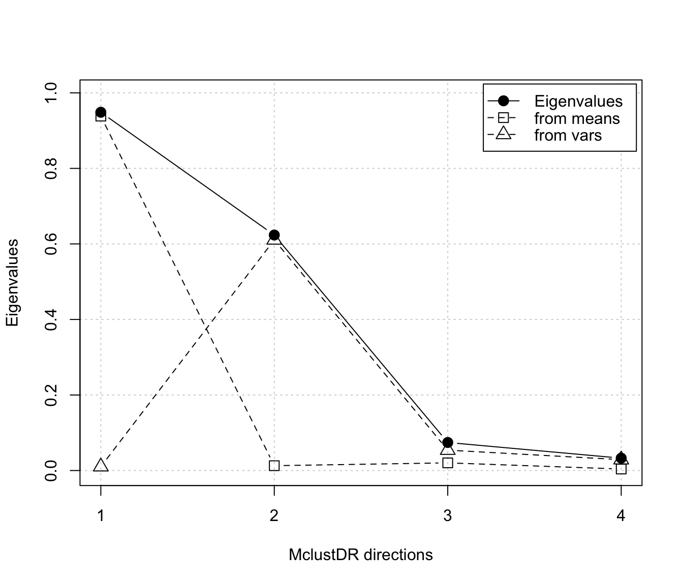
plot(dr, what = "evalues")

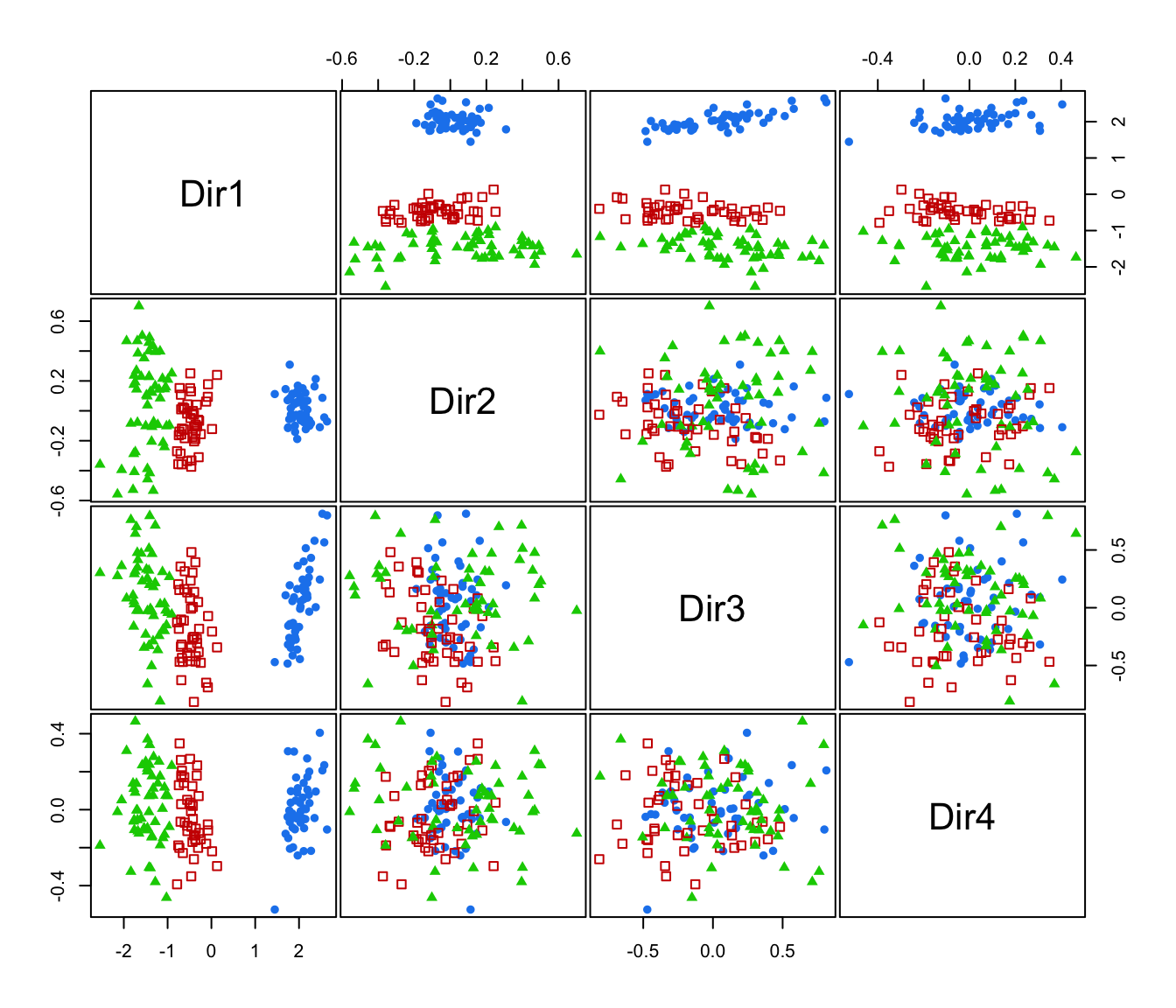
plot(dr, what = "pairs")

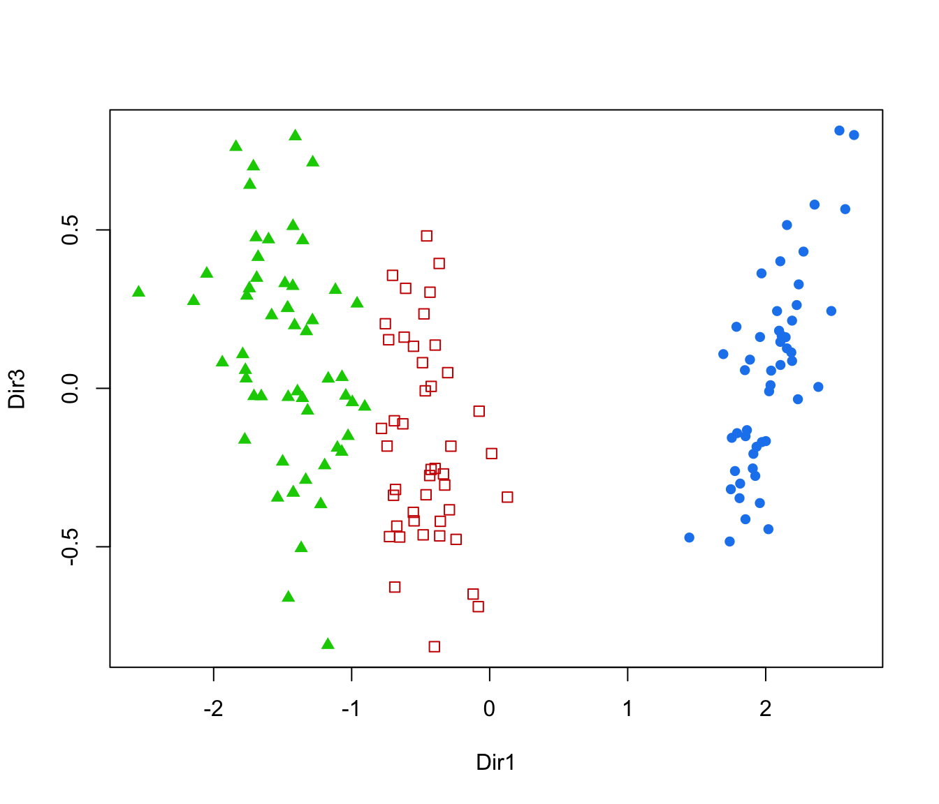
plot(dr, what = "scatterplot", dimens = c(1,3))

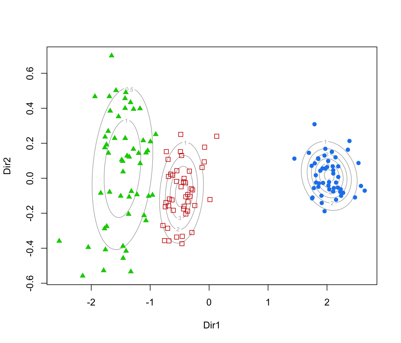
plot(dr, what = "contour")

plot(dr, what = "classification", ngrid = 200)

plot(dr, what = "boundaries", ngrid = 200)

plot(dr, what = "density")

plot(dr, what = "density", dimens = 2)


data(banknote)
da <- MclustDA(banknote[,2:7], banknote$Status, G = 1:3)
dr <- MclustDR(da)
plot(dr, what = "evalues")

plot(dr, what = "pairs")

plot(dr, what = "contour")

plot(dr, what = "classification", ngrid = 200)

plot(dr, what = "boundaries", ngrid = 200)

plot(dr, what = "density")

plot(dr, what = "density", dimens = 2)

# }