3 Model-Based Clustering
\[ \DeclareMathOperator{\Real}{\mathbb{R}} \DeclareMathOperator{\Proj}{\text{P}} \DeclareMathOperator{\Exp}{\text{E}} \DeclareMathOperator{\Var}{\text{Var}} \DeclareMathOperator{\var}{\text{var}} \DeclareMathOperator{\sd}{\text{sd}} \DeclareMathOperator{\cov}{\text{cov}} \DeclareMathOperator{\cor}{\text{cor}} \DeclareMathOperator{\range}{\text{range}} \DeclareMathOperator{\rank}{\text{rank}} \DeclareMathOperator{\ind}{\perp\hspace*{-1.1ex}\perp} \DeclareMathOperator{\CE}{\text{CE}} \DeclareMathOperator{\BS}{\text{BS}} \DeclareMathOperator{\ECM}{\text{ECM}} \DeclareMathOperator{\BSS}{\text{BSS}} \DeclareMathOperator{\WSS}{\text{WSS}} \DeclareMathOperator{\TSS}{\text{TSS}} \DeclareMathOperator{\BIC}{\text{BIC}} \DeclareMathOperator{\ICL}{\text{ICL}} \DeclareMathOperator{\CV}{\text{CV}} \DeclareMathOperator{\diag}{\text{diag}} \DeclareMathOperator{\se}{\text{se}} \DeclareMathOperator{\Cov}{\text{Cov}} \DeclareMathOperator{\boot}{\text{boot}} \DeclareMathOperator{\LRTS}{\text{LRTS}} \DeclareMathOperator{\Model}{\mathcal{M}} \DeclareMathOperator*{\argmin}{arg\min} \DeclareMathOperator*{\argmax}{arg\max} \DeclareMathOperator{\vech}{vech} \DeclareMathOperator{\tr}{tr} \]
This chapter describes the general methodology for Gaussian model-based clustering in mclust, including model estimation and selection. Several data examples are presented, in both the multivariate and univariate case. EM algorithm initialization is discussed at some length, as this is a major issue for model-based clustering. Model-based hierarchical agglomerative clustering is also presented, and the corresponding implementation in mclust is shown. The chapter concludes by providing some details on performing single E- and M- steps, and on control parameters used by the EM functions in mclust.
3.1 Gaussian Mixture Models for Cluster Analysis
Cluster analysis refers to a broad set of multivariate statistical methods and techniques which seek to identify homogeneous subgroups of cases in a dataset, that is, to partition similar observations into meaningful and useful clusters. Cluster analysis is an instance of unsupervised learning, since the presence and number of clusters may not be known a priori, nor is case labeling available.
Many approaches to clustering have been proposed in the literature for exploring the underlying group structure of data. Traditional methods are combinatorial in nature, and either hierarchical (agglomerative or divisive) or non-hierarchical (for example, \(k\)-means). Although some are related to formal statistical models, they typically are based on heuristic procedures which make no explicit assumptions about the structure of the clusters. The choice of clustering method, similarity measures, and interpretation have tended to be informal and often subjective.
Model-based clustering (MBC) is a probabilistic approach to clustering in which each cluster corresponds to a mixture component described by a probability distribution with unknown parameters. The type of distribution is often specified a priori (most commonly Gaussian), whereas the model structure (including the number of components) remains to be determined by parameter estimation and model-selection techniques. Parameters can be estimated by maximum likelihood, using, for instance, the EM algorithm, or by Bayesian approaches. These model-based methods are increasingly favored over heuristic clustering methods. Moreover, the one-to-one relationship between mixture components and clusters can be relaxed, as discussed in Section 7.3.
Model-based clustering can be viewed as a generative approach because it attempts to learn generative models from the data, with each model representing one particular cluster. It is possible to simulate from an estimated model, as discussed in Section 7.4, which can be useful for resampling inference, sensitivity, and predictive analysis.
The finite mixture of Gaussian distributions described in Section 2.2 is one of the most flexible classes of models for continuous variables and, as such, it has become a method of choice in a wide variety of settings. Component covariance matrices can be parameterized by eigen-decomposition to impose geometric constraints, as described in Section 2.2.1. Constraining some but not all of the quantities in Equation 2.4 to be equal between clusters yields parsimonious and easily interpretable models, appropriate for diverse clustering situations. Once the parameters of a Gaussian mixture model (GMM) are estimated via EM, a partition \(\mathcal{C}=\{ C_1, \dots, C_G \}\) of the data into \(G\) clusters can be derived by assigning each observation \(\boldsymbol{x}_i\) to the component with the largest conditional probability that \(\boldsymbol{x}_i\) arises from that component distribution — the MAP principle discussed in Section 2.2.4.
The parameterization includes, but is not restricted to, well-known covariance models that are associated with various criteria for hierarchical clustering: equal-volume spherical variance (sum of squares criterion) (Ward 1963), constant variance (Friedman and Rubin 1967), and unconstrained variance (Scott and Symons 1971). Moreover, \(k\)-means, although it does not make an explicit assumption about the structure of the data, is related to the GMM with spherical, equal volume components (Celeux and Govaert 1995).
3.2 Clustering in mclust
The main function to fit GMMs for clustering is called Mclust(). This function requires a numeric matrix or data frame, with \(n\) observations along the rows and \(d\) variables along the columns, to be supplied as the data argument. In the univariate case (\(d = 1\)), the data can be input as a vector. The number of mixture components \(G\), and the model name corresponding to the eigen-decomposition discussed in Section 2.2.1, can also be specified. By default, all of the available models are estimated for up to \(G=9\) mixture components, but this number can be increased by specifying the argument G accordingly.
Table 3.1 lists the models currently implemented in mclust, both in the univariate and multivariate cases. Options for specification of a noise component and a prior distribution are also shown; these will be discussed in Section 7.1 and Section 7.2, respectively.
| Label | Model | Distribution | HC | GMM | GMM + noise | GMM + prior |
|---|---|---|---|---|---|---|
X |
\(\sigma^2\) | Univariate | ✓ | ✓ | ✓ | |
E |
\(\sigma^2\) | Univariate | ✓ | ✓ | ✓ | ✓ |
V |
\(\sigma_k^2\) | Univariate | ✓ | ✓ | ✓ | ✓ |
XII |
\(\diag(\sigma^2, \ldots, \sigma^2)\) | Spherical | ✓ | ✓ | ✓ | |
XXI |
\(\diag(\sigma_1^2, \ldots, \sigma_d^2)\) | Diagonal | ✓ | ✓ | ✓ | |
XXX |
\(\boldsymbol{\Sigma}\) | Ellipsoidal | ✓ | ✓ | ✓ | |
EII |
\(\lambda \boldsymbol{I}\) | Spherical | ✓ | ✓ | ✓ | ✓ |
VII |
\(\lambda_k \boldsymbol{I}\) | Spherical | ✓ | ✓ | ✓ | ✓ |
EEI |
\(\lambda \boldsymbol{\Delta}\) | Diagonal | ✓ | ✓ | ✓ | |
VEI |
\(\lambda_k \boldsymbol{\Delta}\) | Diagonal | ✓ | ✓ | ✓ | |
EVI |
\(\lambda \boldsymbol{\Delta}_k\) | Diagonal | ✓ | ✓ | ✓ | |
VVI |
\(\lambda_k \boldsymbol{\Delta}_k\) | Diagonal | ✓ | ✓ | ✓ | |
EEE |
\(\lambda \boldsymbol{U}\boldsymbol{\Delta}\boldsymbol{U}{}^{\!\top}\) | Ellipsoidal | ✓ | ✓ | ✓ | ✓ |
VEE |
\(\lambda_k \boldsymbol{U}\boldsymbol{\Delta}\boldsymbol{U}{}^{\!\top}\) | Ellipsoidal | ✓ | ✓ | ||
EVE |
\(\lambda \boldsymbol{U}\boldsymbol{\Delta}_k \boldsymbol{U}{}^{\!\top}\) | Ellipsoidal | ✓ | ✓ | ||
VVE |
\(\lambda_k \boldsymbol{U}\boldsymbol{\Delta}_k \boldsymbol{U}{}^{\!\top}\) | Ellipsoidal | ✓ | ✓ | ||
EEV |
\(\lambda \boldsymbol{U}_k \boldsymbol{\Delta}\boldsymbol{U}{}^{\!\top}_k\) | Ellipsoidal | ✓ | ✓ | ✓ | |
VEV |
\(\lambda_k \boldsymbol{U}_k \boldsymbol{\Delta}\boldsymbol{U}{}^{\!\top}_k\) | Ellipsoidal | ✓ | ✓ | ✓ | |
EVV |
\(\lambda \boldsymbol{U}_k \boldsymbol{\Delta}_k \boldsymbol{U}{}^{\!\top}_k\) | Ellipsoidal | ✓ | ✓ | ||
VVV |
\(\lambda_k \boldsymbol{U}_k \boldsymbol{\Delta}_k \boldsymbol{U}{}^{\!\top}_k\) | Ellipsoidal | ✓ | ✓ | ✓ | ✓ |
The diagram in Figure 3.1 presents the flow chart of the model-based clustering approach implemented in the function Mclust() of the mclust package.
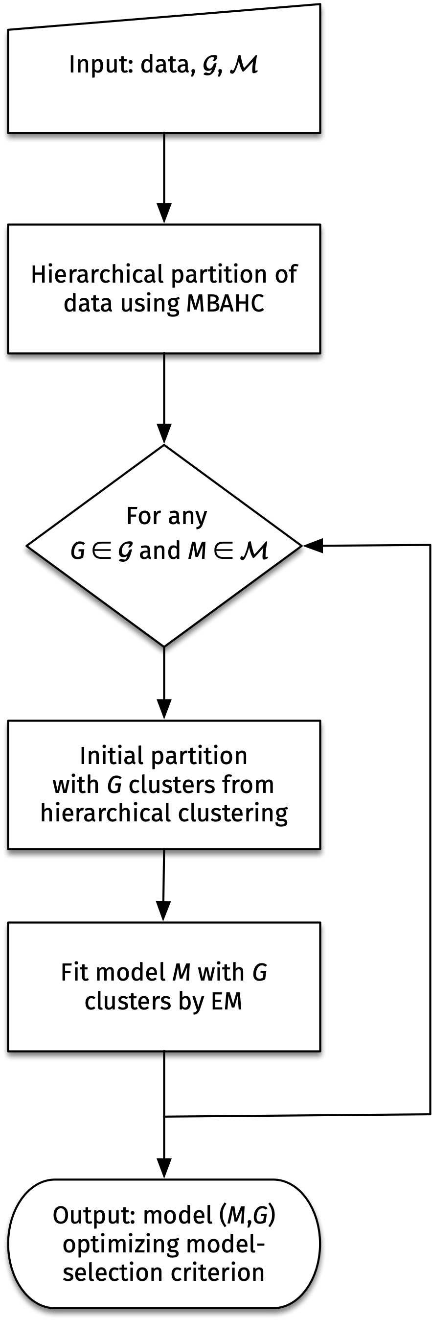
Given numerical data, a model-based agglomerative hierarchical clustering (MBAHC) procedure is first applied, for which details are given in Section 3.6. For a set \(\mathcal{G}\) giving the numbers of mixture components to consider, and a list \(\mathcal{M}\) of models with within-cluster covariance eigen-decomposition chosen from Table 3.1, the hierarchical partitions obtained for any number of components in the set \(\mathcal{G}\) are used to start the EM algorithm. GMMs are then fit for any combination of elements \(G \in \mathcal{G}\) and \(M \in \mathcal{M}\). At the end of the procedure, the model with the best value of the model-selection criterion is returned (BIC is the default for model selection; see {#sec-modsel_cluster} for available options).
Example 3.1 Clustering diabetes data
The diabetes dataset from Reaven and Miller (1979), available in the R package rrcov (Todorov 2022), contains measurements on 145 non-obese adult subjects. A description of the variables is given in the table below.
| Variable | Description |
|---|---|
rw |
Relative weight, expressed as the ratio of actual weight to expected weight, given the subject’s height. |
fpg |
Fasting plasma glucose level. |
glucose |
Area under the plasma glucose curve. |
insulin |
Area under the plasma insulin curve. |
sspg |
Steady state plasma glucose level, a measure of insulin resistance. |
The glucose and insulin measurements were recorded for a three hour oral glucose tolerance test (OGTT). The subjects are clinically classified into three groups: "normal", "overt" diabetes (the most advanced stage), and "chemical" diabetes (a latent stage preceding overt diabetes).
The data can be shown graphically as in Figure 3.2 with the following code:
clp = clPairs(X, Class, lower.panel = NULL)
clPairsLegend(0.1, 0.3, class = clp$class, col = clp$col, pch = clp$pch)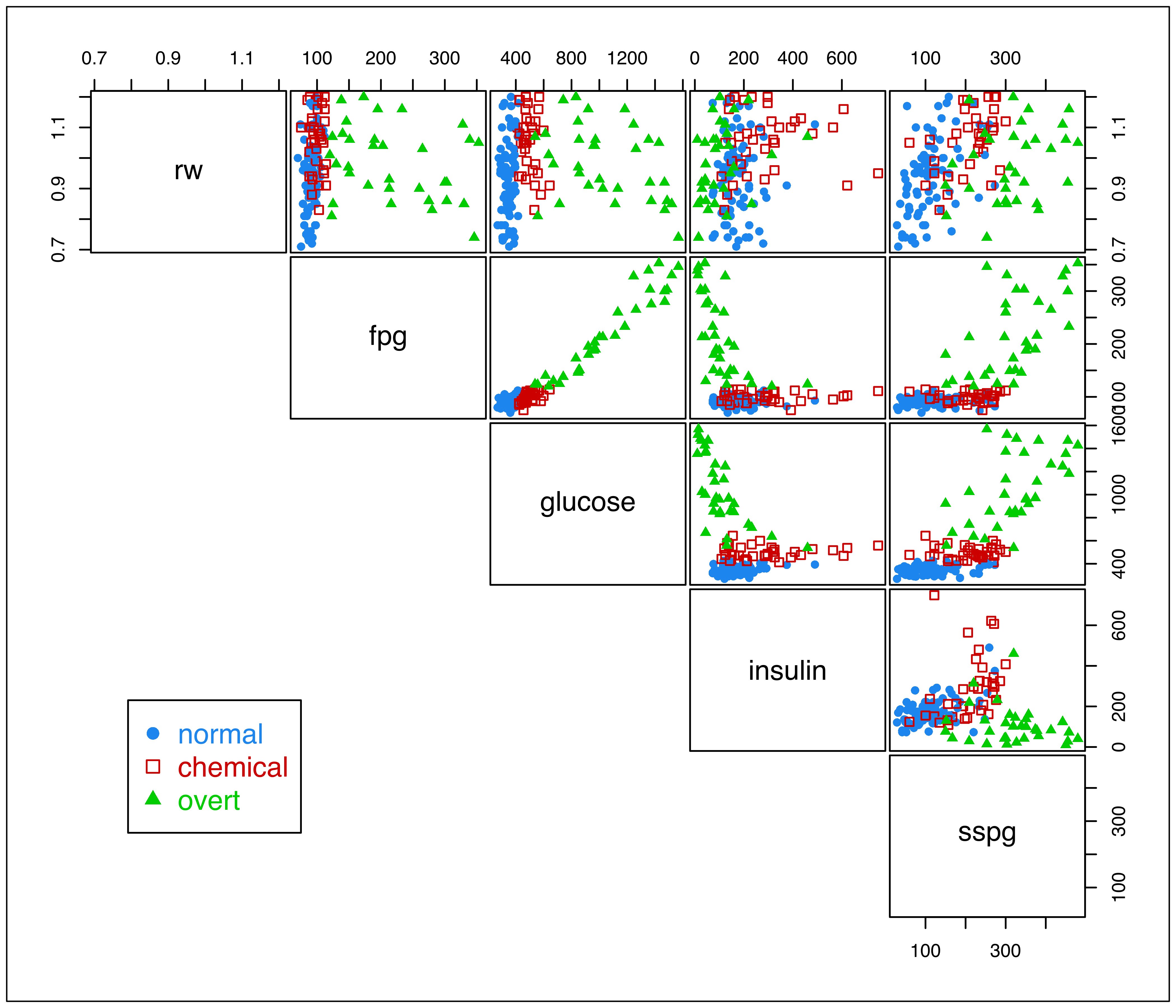
diabetes data with points marked according to the true classification.
The clPairs() function is an enhanced version of the base pairs() function, which allows data points to be represented by different colors and symbols. The function invisibly returns a list information useful for adding a legend via the clPairsLegend() function.
The following command performs a cluster analysis of the diabetes dataset for an unconstrained covariance model (VVV in the nomenclature of Table 2.1 and Table 3.1) with three mixture components:
mod = Mclust(X, G = 3, modelNames = "VVV")Next, a summary of the modeling results is printed:
summary(mod)
## ----------------------------------------------------
## Gaussian finite mixture model fitted by EM algorithm
## ----------------------------------------------------
##
## Mclust VVV (ellipsoidal, varying volume, shape, and orientation) model
## with 3 components:
##
##  log-likelihood   n df     BIC     ICL
##         -2936.8 145 62 -6182.2 -6189.5
##
## Clustering table:
##  1  2  3
## 78 40 27
By adding the optional argument parameters = TRUE, a more detailed summary can be obtained, including the estimated parameters:
summary(mod, parameters = TRUE)
## ----------------------------------------------------
## Gaussian finite mixture model fitted by EM algorithm
## ----------------------------------------------------
##
## Mclust VVV (ellipsoidal, varying volume, shape, and orientation) model
## with 3 components:
##
##  log-likelihood   n df     BIC     ICL
##         -2936.8 145 62 -6182.2 -6189.5
##
## Clustering table:
##  1  2  3
## 78 40 27
##
## Mixing probabilities:
##       1       2       3
## 0.53635 0.27605 0.18760
##
## Means:
##              [,1]     [,2]       [,3]
## rw        0.93884   1.0478    0.98353
## fpg      91.76513 102.9543  236.39448
## glucose 357.21471 508.7962 1127.76651
## insulin 166.14835 298.1248   78.38848
## sspg    107.47991 228.7259  338.06062
##
## Variances:
## [,,1]
##                 rw      fpg   glucose      insulin      sspg
## rw       0.0160109   0.3703    1.7519   -0.0072541    2.5199
## fpg      0.3703007  63.8795  128.5895   29.8548772   58.8162
## glucose  1.7518634 128.5895 2090.3853  269.2839704  408.9926
## insulin -0.0072541  29.8549  269.2840 2656.1047748  856.5919
## sspg     2.5198642  58.8162  408.9926  856.5919127 2131.0809
## [,,2]
##                rw        fpg    glucose    insulin       sspg
## rw       0.011785   -0.25403    -2.4794     1.7088     2.2958
## fpg     -0.254030  210.19848  1035.1415  -242.8201   -74.2975
## glucose -2.479438 1035.14145  8151.8109 -1301.0449 -1021.8653
## insulin  1.708775 -242.82013 -1301.0449 24803.2354  2202.7878
## sspg     2.295790  -74.29753 -1021.8653  2202.7878  2453.5726
## [,,3]
##                 rw        fpg   glucose    insulin      sspg
## rw        0.013712    -3.1314   -16.683     2.7459    3.2804
## fpg      -3.131374  4910.7530 17669.044 -2208.7550 2630.6654
## glucose -16.682509 17669.0438 71474.571 -9214.1986 9005.4355
## insulin   2.745916 -2208.7550 -9214.199  2124.2757 -296.8184
## sspg      3.280440  2630.6654  9005.435  -296.8184 6392.4694
The following table shows the relationship between the true classes and those defined by the fitted GMM:
table(Class, Cluster = mod$classification)
##           Cluster
## Class       1  2  3
##   normal   70  6  0
##   chemical  8 28  0
##   overt     0  6 27
adjustedRandIndex(Class, mod$classification)
## [1] 0.65015
Roughly, the first cluster appears to be associated with normal subjects, the second cluster with chemical diabetes, and the last cluster with subjects suffering from overt diabetes. Also shown is the adjusted Rand index (ARI, Hubert and Arabie 1985), which can be used for evaluating a clustering solution. The ARI is a measure of agreement between two partitions, one that is estimated by a statistical procedure ignoring the labeling of the groups and the other that is the true classification. It has zero expected value in the case of a random partition, corresponding to the hypothesis of independent clusterings with fixed marginals, and is bounded above by 1, with higher values representing better partition accuracy. In this case, a better classification could be obtained by including the full range of available covariance models (the default) in the call to Mclust().
The plot() method associated with Mclust() provides for a variety of displays. For instance, the following code produces a plot showing the clustering partition derived from the fitted GMM:
plot(mod, what = "classification")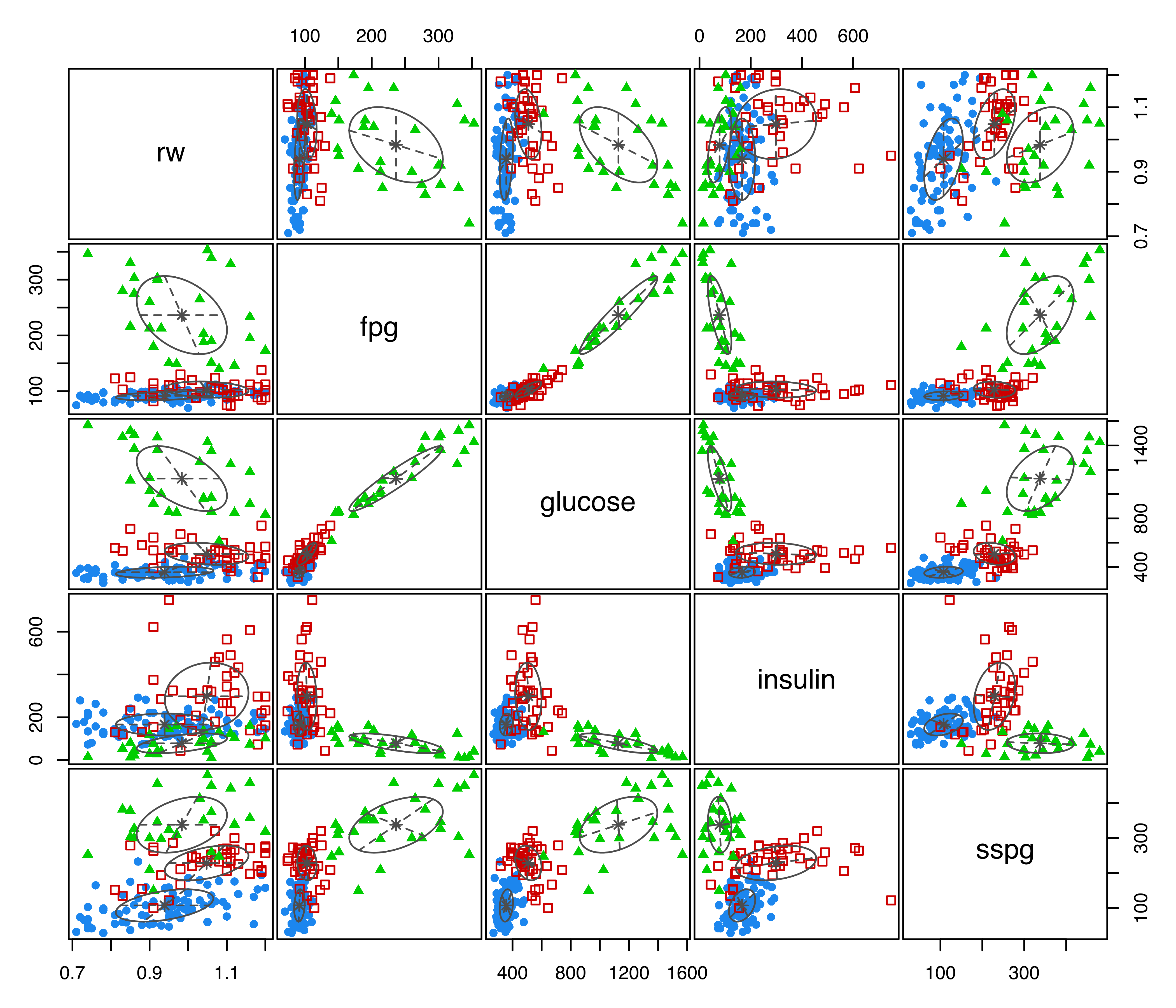
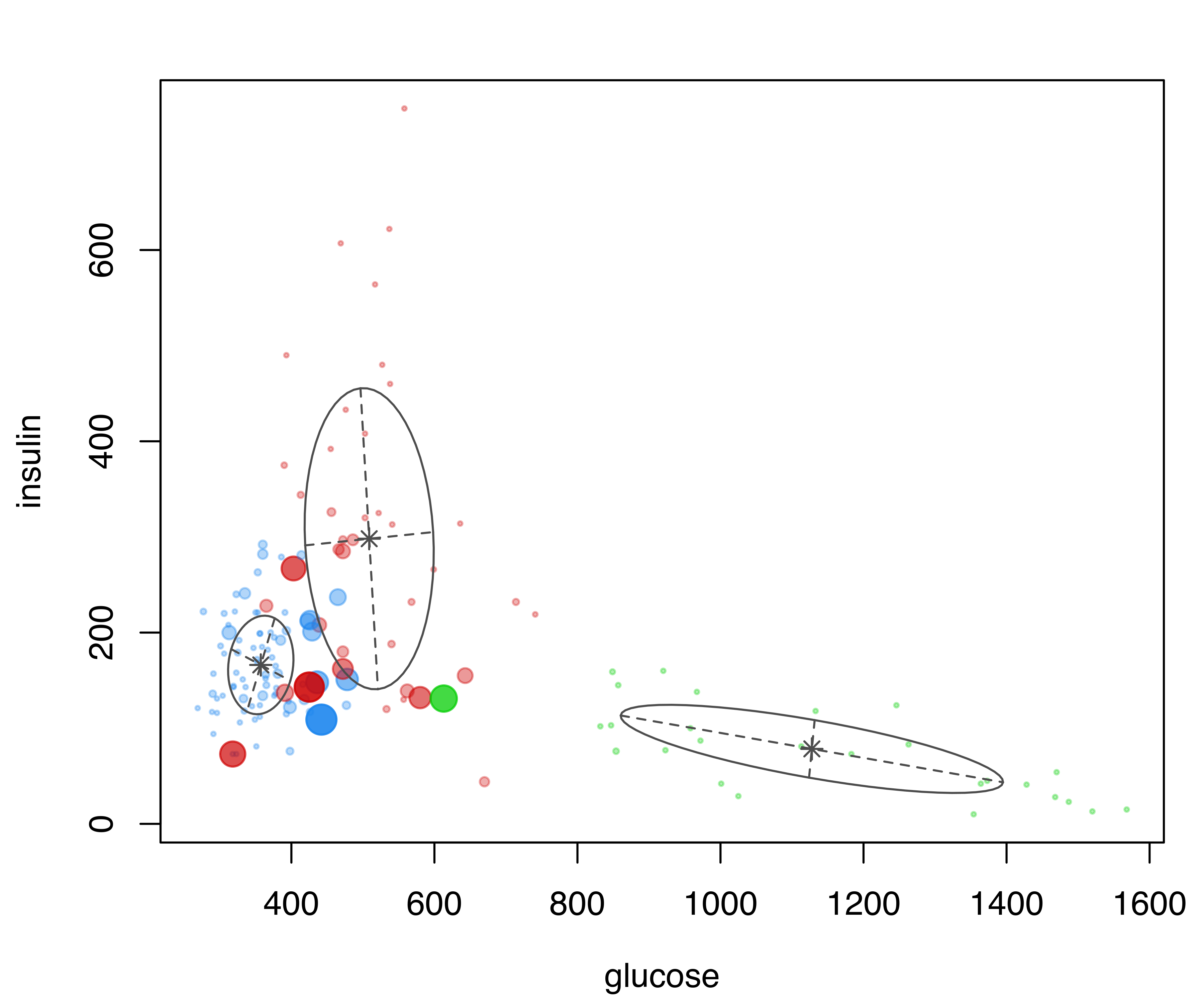
diabetes data with points colored according to the mclust classification, and ellipses corresponding to projections of the mclust cluster covariances.
The resulting plot is shown in Figure 3.3, with points marked on the basis of the MAP classification (see Section 2.2.4), and ellipses showing the projection of the two-dimensional analog of the standard deviation for the cluster covariances of the estimated GMM. The ellipses can be dropped by specifying the optional argument addEllipses = FALSE, and filled ellipses can be obtained with the code:
plot(mod, what = "classification", fillEllipses = TRUE)The previous figures showed scatterplot matrices of all pairs of variables. A subset of pairs plots can be specified using the optional argument dimen. For instance, the following code selects the first two variables (see Figure 3.4):
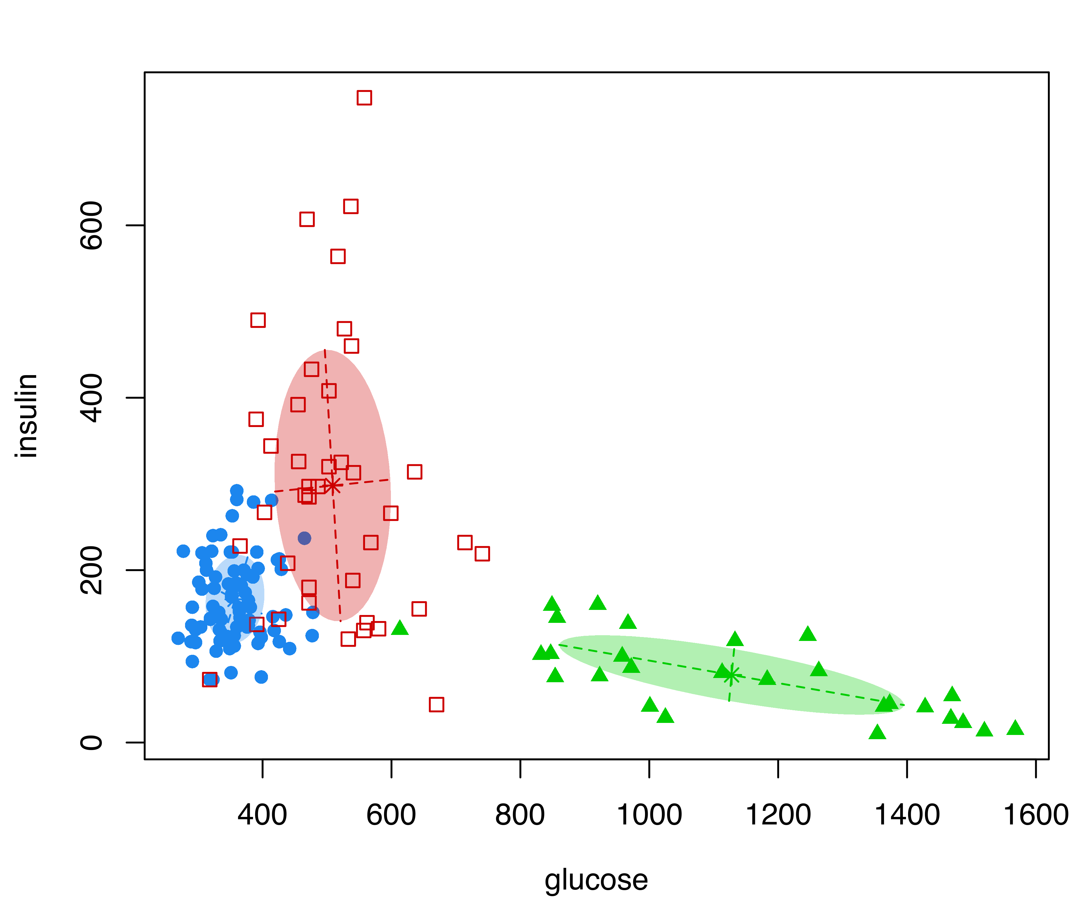
diabetes data with points marked according to the mclust classification, and filled ellipses corresponding to mclust cluster covariances.
Uncertainty associated with the MAP classification (see Section 2.2.4) can also be represented graphically as follows:
diabetes data with points marked according to the clustering, and point size reflecting the corresponding uncertainty of the MAP classification for the mclust model.
The resulting plot is shown in Figure 3.5, where the size of the data points reflects the classification uncertainty. Subsets of variables can also be specified for this type of graph.
Plots can be selected interactively by leaving the what argument unspecified, in which case the plot() function will supply a menu of options. Chapter 6 provides a more detailed description of the graphical capabilities available in mclust for further fine-tuning.
Example 3.2 Clustering thyroid disease data
Consider the thyroid disease data (Coomans and Broeckaert 1986) that provides the results of five laboratory tests administered to a sample of 215 patients. The tests are used to predict whether a patient’s thyroid can be classified as euthyroidism (normal thyroid gland function), hypothyroidism (underactive thyroid not producing enough thyroid hormone) or hyperthyroidism (overactive thyroid producing and secreting excessive amounts of the free thyroid hormones T3 and/or thyroxine T4). Diagnosis of thyroid function was based on a complete medical record, including anamnesis, scan, and other measurements.
The data is one of several datasets included in the “Thyroid Disease Data Set” of the UCI Machine Learning Repository (Dua and Graff (2017) — see https://archive.ics.uci.edu/ml/datasets/thyroid+disease). The data used here, which corresponds to new-thyroid.data and new-thyroid.names in the data folder at the UCI site, is available as a dataset in mclust. A description of the variables is given in the table below, and a plot of the data is shown in Figure 3.6.
| Variable | Description |
|---|---|
Diagnosis |
Diagnosis of thyroid operation: Hypo, Normal, and Hyper. |
RT3U |
T3-resin uptake test (percentage). |
T4 |
Total serum thyroxin as measured by the isotopic displacement method. |
T3 |
Total serum triiodothyronine as measured by radioimmuno assay. |
TSH |
Basal thyroid-stimulating hormone (TSH) as measured by radioimmuno assay. |
DTSH |
Maximal absolute difference of TSH value after injection of 200 micro grams of thyrotropin-releasing hormone as compared to the basal value. |
data("thyroid", package = "mclust")
X = data.matrix(thyroid[, 2:6])
Class = thyroid$Diagnosis

clp = clPairs(X, Class, lower.panel = NULL,
              symbols = c(0, 1, 2),
              colors = c("gray50", "black", "red3"))
clPairsLegend(0.1, 0.3, title = "Thyroid diagnosis:", class = clp$class,
              col = clp$col, pch = clp$pch)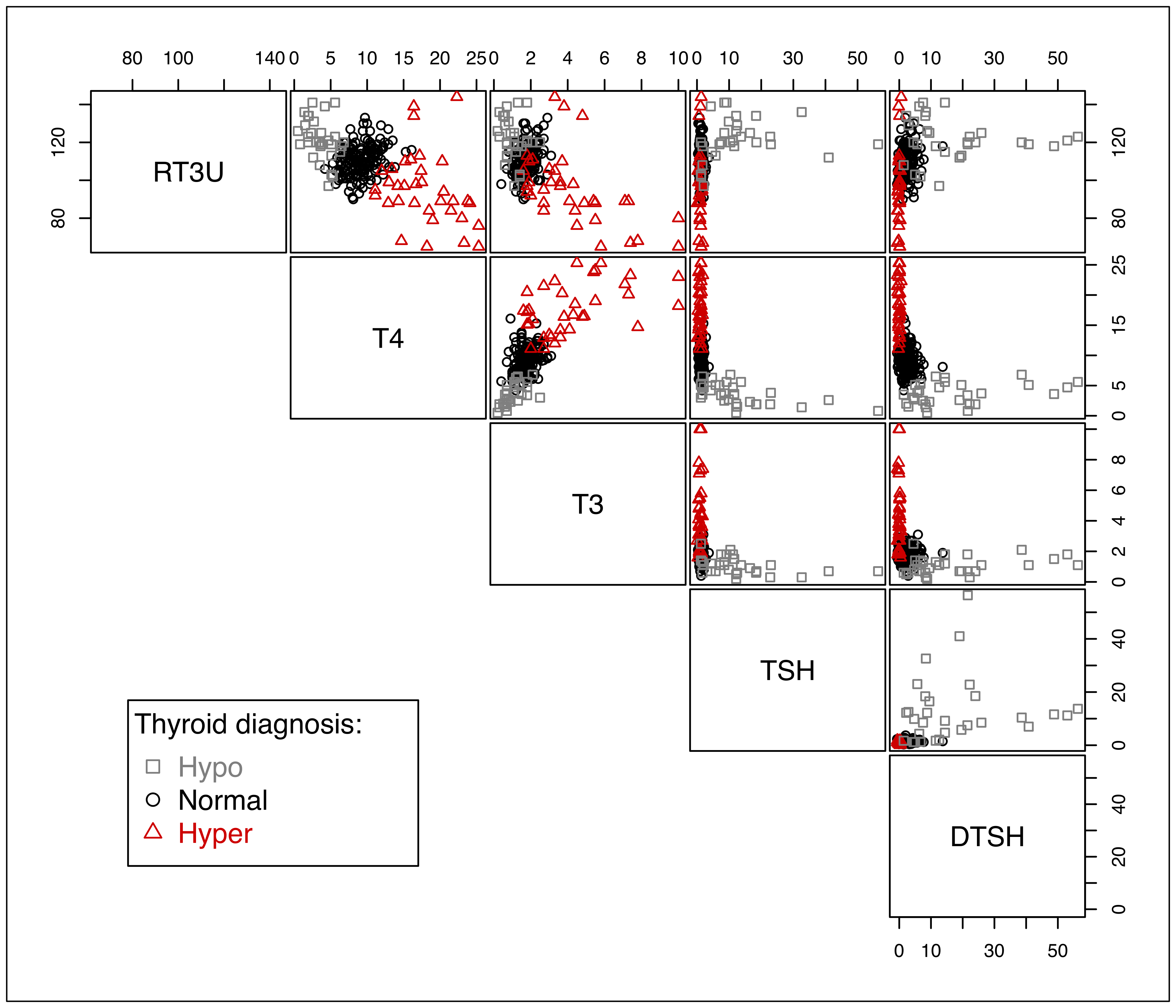
thyroid gland data.
In Example 3.1 we fitted a GMM by specifying both the numbers of mixture components to be considered, using the argument G, and the models for the component-covariance matrices to be used, using the argument modelNames. Users can provide multiple values for both arguments, a vector of integers for G, a vector of character strings for modelNames. By default, G = 1:9, so GMMs with up to nine components are fitted, and all of the available models shown in Table 3.1 are used for modelNames.
Clustering of the thyroid data is obtained using the following R command:
mod = Mclust(X)Since we have provided only the data in the function call, selection of both the number of mixture components and the covariance parameterization is done automatically using the default model selection criterion, BIC. We can inspect the table of BIC values for all the \(9 \times 14 = 126\) estimated models as follows:
mod$BIC
## Bayesian Information Criterion (BIC):
##       EII     VII     EEI     VEI     EVI     VVI     EEE     VEE
## 1 -7477.4 -7477.4 -6699.7 -6699.7 -6699.7 -6699.7 -6388.4 -6388.4
## 2 -7265.4 -6780.9 -6399.7 -5475.4 -5446.6 -5276.3 -6231.3 -5429.6
## 3 -6971.3 -6404.0 -6081.2 -5471.7 -5110.3 -4777.9 -6228.4 -5273.3
## 4 -6726.5 -6263.1 -5972.8 -5281.3 -5146.0 -4796.8 -6260.7 -5381.4
## 5 -6604.0 -6077.5 -5920.8 -5248.8 -4897.4 -4810.9 -6292.6 -5276.0
## 6 -6574.1 -6002.9 -5893.5 -5230.1 -4945.0 -4854.6 -5946.0 -5291.6
## 7 -6572.8 -5967.0 -6116.2 -5250.0 -4960.5 -4860.0 -5977.3 -5279.3
## 8 -6500.2 -5947.6 -6065.9 -5253.0 -5003.5 -4881.4 -5924.7 -5327.2
## 9 -6370.8 -5904.0 -5579.3 -5244.5 -5089.2 -4876.4 -5696.2 -5273.0
##       EVE     VVE     EEV     VEV     EVV     VVV
## 1 -6388.4 -6388.4 -6388.4 -6388.4 -6388.4 -6388.4
## 2 -5286.3 -5163.6 -5354.9 -5166.4 -5241.5 -5150.8
## 3 -5036.4 -5453.9 -5272.8 -5181.0 -5048.4 -4809.8
## 4 -4974.8 -5478.8 -5129.3 -4902.6 -5061.9 -5175.3
## 5 -5022.6 -5474.2 -5233.9 -4972.1      NA -4959.9
## 6 -4932.2 -4878.3 -5290.6 -5005.4 -5141.0 -5012.5
## 7 -5039.8 -4888.7 -5359.3 -5209.3 -5250.2 -5096.8
## 8 -5086.9 -4909.7 -5376.2 -5070.9 -5347.1 -5129.7
## 9      NA      NA -5287.7 -5091.2      NA      NA
##
## Top 3 models based on the BIC criterion:
##   VVI,3   VVI,4   VVV,3
## -4777.9 -4796.8 -4809.8
The missing values (denoted by NA) that appear in the BIC table indicate that a particular model could not be estimated as initialized. This usually happens when a covariance matrix estimate becomes singular during EM. The Bayesian regularization method proposed by Fraley and Raftery (2007) and implemented in mclust as described in Section 7.2 addresses this problem.
The top three models are also listed at the bottom of the table. A summary of the top models according to the BIC criterion can also be obtained as
summary(mod$BIC, k = 5)
## Best BIC values:
##            VVI,3     VVI,4     VVV,3     VVI,5     VVI,6
## BIC      -4777.9 -4796.773 -4809.761 -4810.928 -4854.644
## BIC diff     0.0   -18.866   -31.854   -33.021   -76.737
where we have specified that the the top five GMMs should be shown through the optional argument k = 5. This summary is useful because it provides the BIC differences with respect to the best model, namely, the one with the largest BIC. For the interpretation of BIC, see the discussion in Section 2.3.1.
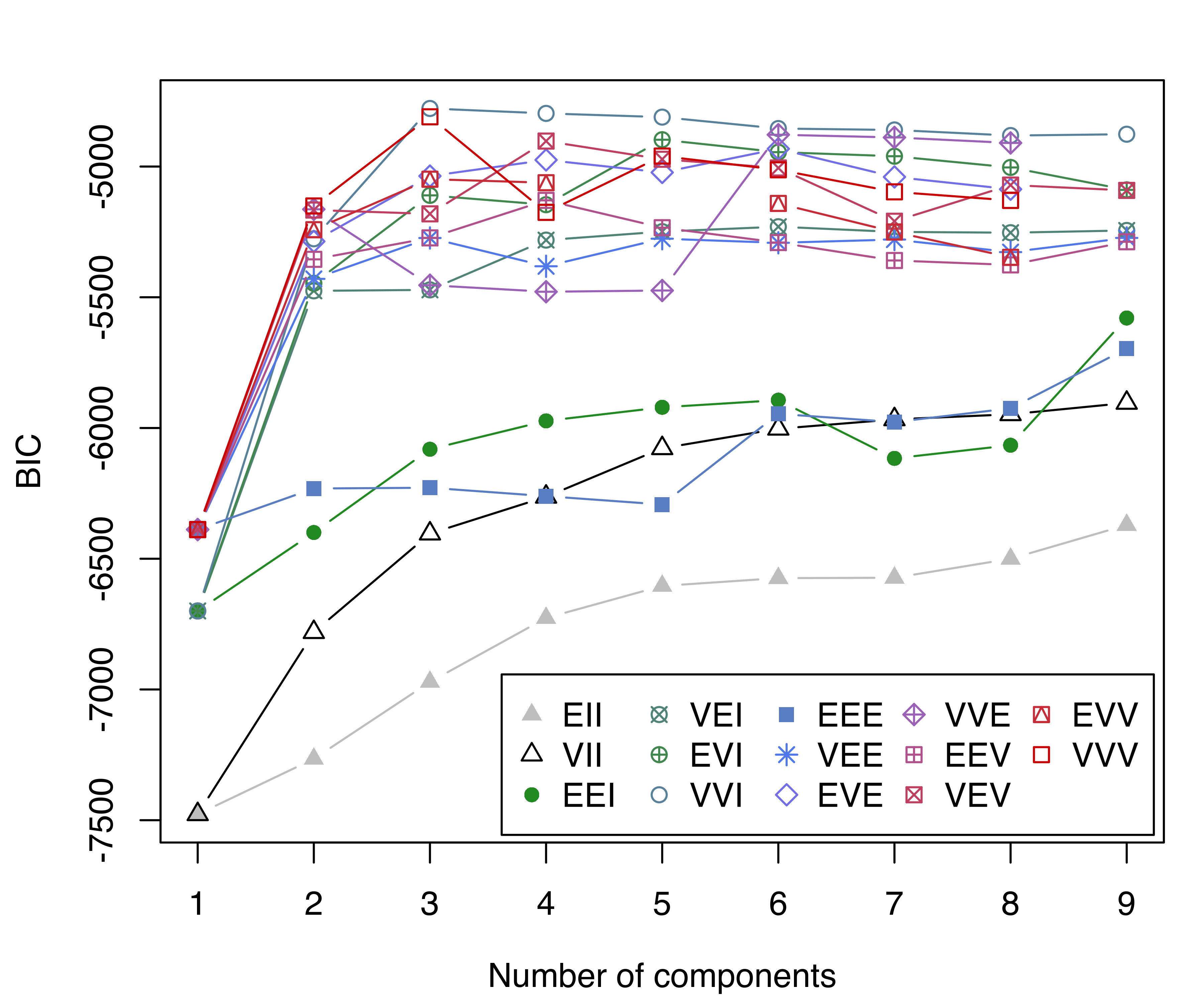
The BIC values can be displayed graphically using
thyroid data.
where we included the optional argument legendArgs to control the placement and format of the legend. The resulting plot of BIC traces is shown in Figure 3.7.
The model selected is (VVI,3), a three-component Gaussian mixture with diagonal covariance structure, in which both the volume and shape vary between clusters. We can obtain a full summary of the model estimates as follows:
summary(mod, parameters = TRUE)
## ----------------------------------------------------
## Gaussian finite mixture model fitted by EM algorithm
## ----------------------------------------------------
##
## Mclust VVI (diagonal, varying volume and shape) model with 3
## components:
##
##  log-likelihood   n df     BIC     ICL
##           -2303 215 32 -4777.9 -4784.5
##
## Clustering table:
##   1   2   3
##  35 152  28
##
## Mixing probabilities:
##       1       2       3
## 0.16310 0.70747 0.12943
##
## Means:
##           [,1]     [,2]     [,3]
## RT3U 95.536865 110.3462 123.2078
## T4   17.678383   9.0880   3.7994
## T3    4.262681   1.7218   1.0576
## TSH   0.970155   1.3051  13.8951
## DTSH -0.017415   2.4960  18.8221
##
## Variances:
## [,,1]
##        RT3U     T4     T3     TSH     DTSH
## RT3U 343.92  0.000 0.0000 0.00000 0.000000
## T4     0.00 17.497 0.0000 0.00000 0.000000
## T3     0.00  0.000 4.9219 0.00000 0.000000
## TSH    0.00  0.000 0.0000 0.15325 0.000000
## DTSH   0.00  0.000 0.0000 0.00000 0.071044
## [,,2]
##        RT3U     T4      T3     TSH   DTSH
## RT3U 66.372 0.0000 0.00000 0.00000 0.0000
## T4    0.000 4.8234 0.00000 0.00000 0.0000
## T3    0.000 0.0000 0.23278 0.00000 0.0000
## TSH   0.000 0.0000 0.00000 0.21394 0.0000
## DTSH  0.000 0.0000 0.00000 0.00000 3.1892
## [,,3]
##       RT3U    T4      T3 TSH   DTSH
## RT3U 95.27 0.000 0.00000   0   0.00
## T4    0.00 4.278 0.00000   0   0.00
## T3    0.00 0.000 0.27698   0   0.00
## TSH   0.00 0.000 0.00000 147   0.00
## DTSH  0.00 0.000 0.00000   0 231.29
The clustering implied by the selected model can then be shown graphically as in Figure 3.8 with the code:
plot(mod, what = "classification")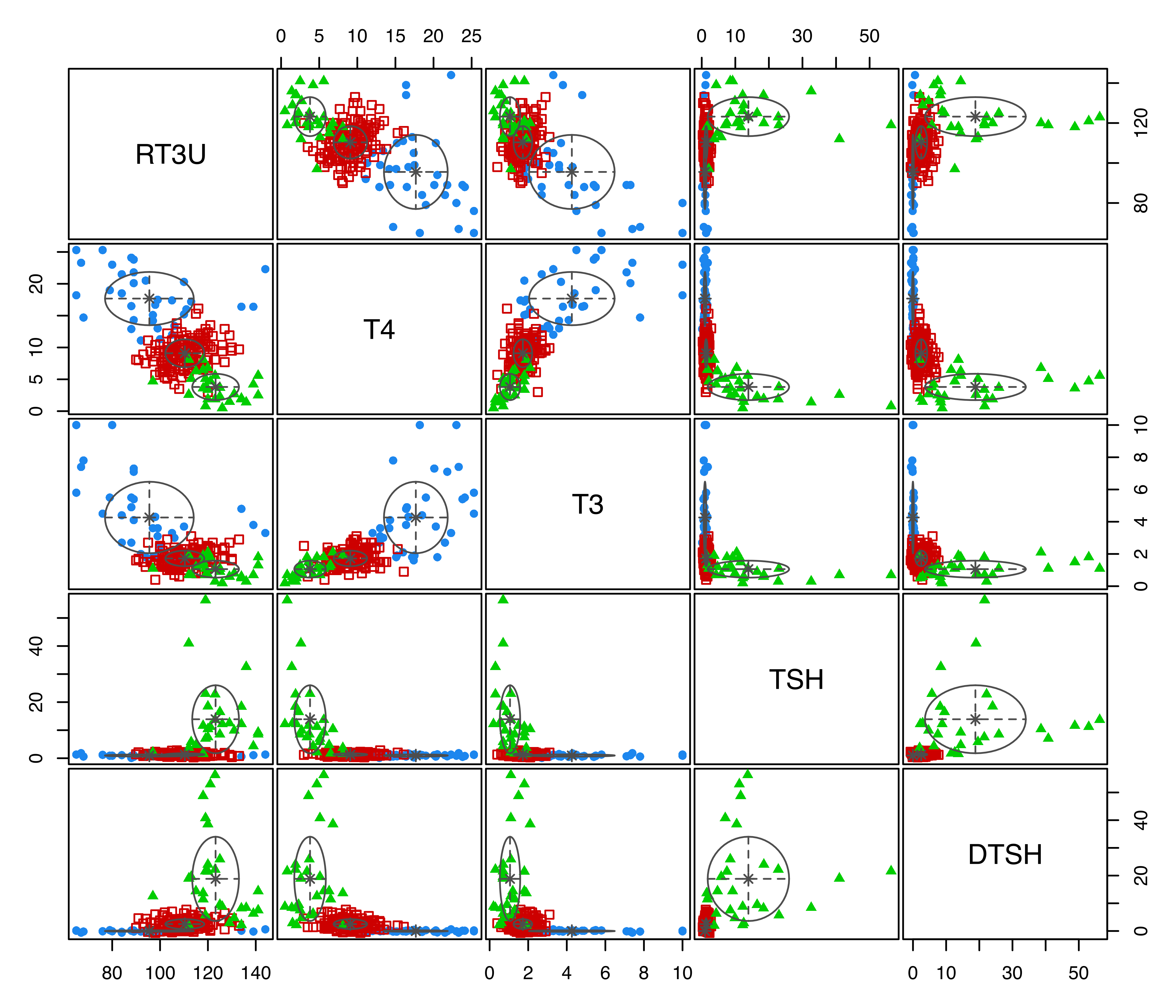
thyroid data with points marked according to the GMM (VVI,3) clustering, and ellipses corresponding to projections of the estimated cluster covariances.
The confusion matrix for the clustering and the corresponding adjusted Rand index are obtained as:
table(Class, Cluster = mod$classification)
##         Cluster
## Class      1   2   3
##   Hypo     0   4  26
##   Normal   1 147   2
##   Hyper   34   1   0
adjustedRandIndex(Class, mod$classification)
## [1] 0.87715
The estimated clustering model turns out to be quite accurate in recovering the true thyroid diagnosis.
A plot of the posterior conditional probabilities ordered by cluster can be obtained using the following code:
z  = mod$z               # posterior conditional probabilities
cl = mod$classification  # MAP clustering
G  = mod$G               # number of clusters
sclass = 10 # class separation
sedge = 3   # edge spacing
L = nrow(z) + G*(sclass+2*sedge)
plot(1:L, runif(L), ylim = c(0, 1), type = "n", axes = FALSE,
     ylab = "Posterior conditional probabilities", xlab = "")
axis(2)
col = mclust.options("classPlotColors")
l = sclass
for (k in 1:G)
{
 i = which(cl == k)
 ord = i[order(z[i, k], decreasing = TRUE)]
 for (j in 1:G)
    points((l+sedge)+1:length(i), z[ord, j],
           pch = as.character(j), col = col[j])
 rect(l, 0, l+2*sedge+length(i), 1,
      border = col[k], col = col[k], lwd = 2, density = 0)
 l = l + 2*sedge + length(i) + sclass
}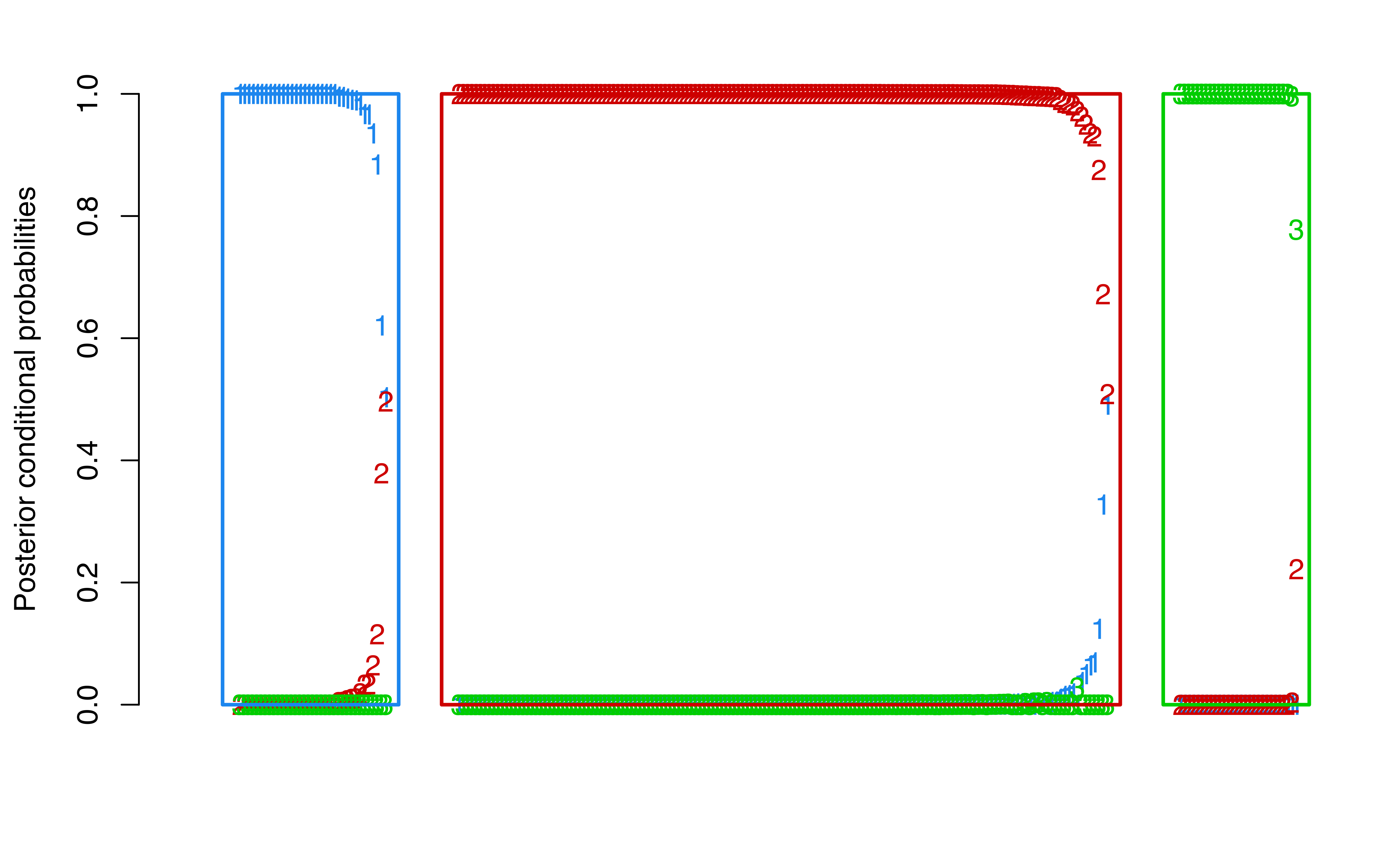
thyroid data. The panels correspond to the different clusters.
This yields Figure 3.9, in which a panel of posterior conditional probabilities of class membership is shown for each of the three clusters determined by the MAP classification. The plot shows that observations in the third cluster have the largest probabilities of membership, while there is some uncertainty in membership among the first two clusters.
Example 3.3 Clustering Italian wines data
Forina et al. (1986) reported data on 178 wines grown in the same region in Italy but derived from three different cultivars (Barbera, Barolo, Grignolino). For each wine, 13 measurements of chemical and physical properties were made as reported in the table below. This data set is from the UCI Machine Learning Data Repository (Dua and Graff (2017) — see http://archive.ics.uci.edu/ml/datasets/Wine) and is available in the gclus package (Hurley 2019).
| Variable | Description |
|---|---|
Class |
Wine classes: 1) Barolo; 2) Grignolino; 3) Barbera |
Alcohol |
Alcohol |
Malic |
Malic acid |
Ash |
Ash |
Alcalinity |
Alcalinity of ash |
Magnesium |
Magnesium |
Phenols |
Total phenols |
Flavanoids |
Flavanoids |
Nonflavanoid |
Nonflavanoid phenols |
Proanthocyanins |
Proanthocyanins |
Intensity |
Color intensity |
Hue |
Hue |
OD280 |
OD280/OD315 of diluted wines |
Proline |
Proline |
data("wine", package = "gclus")
Class = factor(wine$Class, levels = 1:3,
               labels = c("Barolo", "Grignolino", "Barbera"))
X = data.matrix(wine[, -1])
For a description of the data, see help("wine", package = "gclus").
We fit the data with Mclust() for all 14 models, and then summarize the BIC for the top 3 models:
mod = Mclust(X)
summary(mod$BIC, k = 3)
## Best BIC values:
##            VVE,3     EVE,4     VVE,4
## BIC      -6849.4 -6873.616 -6885.472
## BIC diff     0.0   -24.225   -36.081
The BIC traces are then plotted (see Figure 3.10):
plot(mod, what = "BIC",
     ylim = range(mod$BIC[, -(1:2)], na.rm = TRUE),
     legendArgs = list(x = "bottomleft"))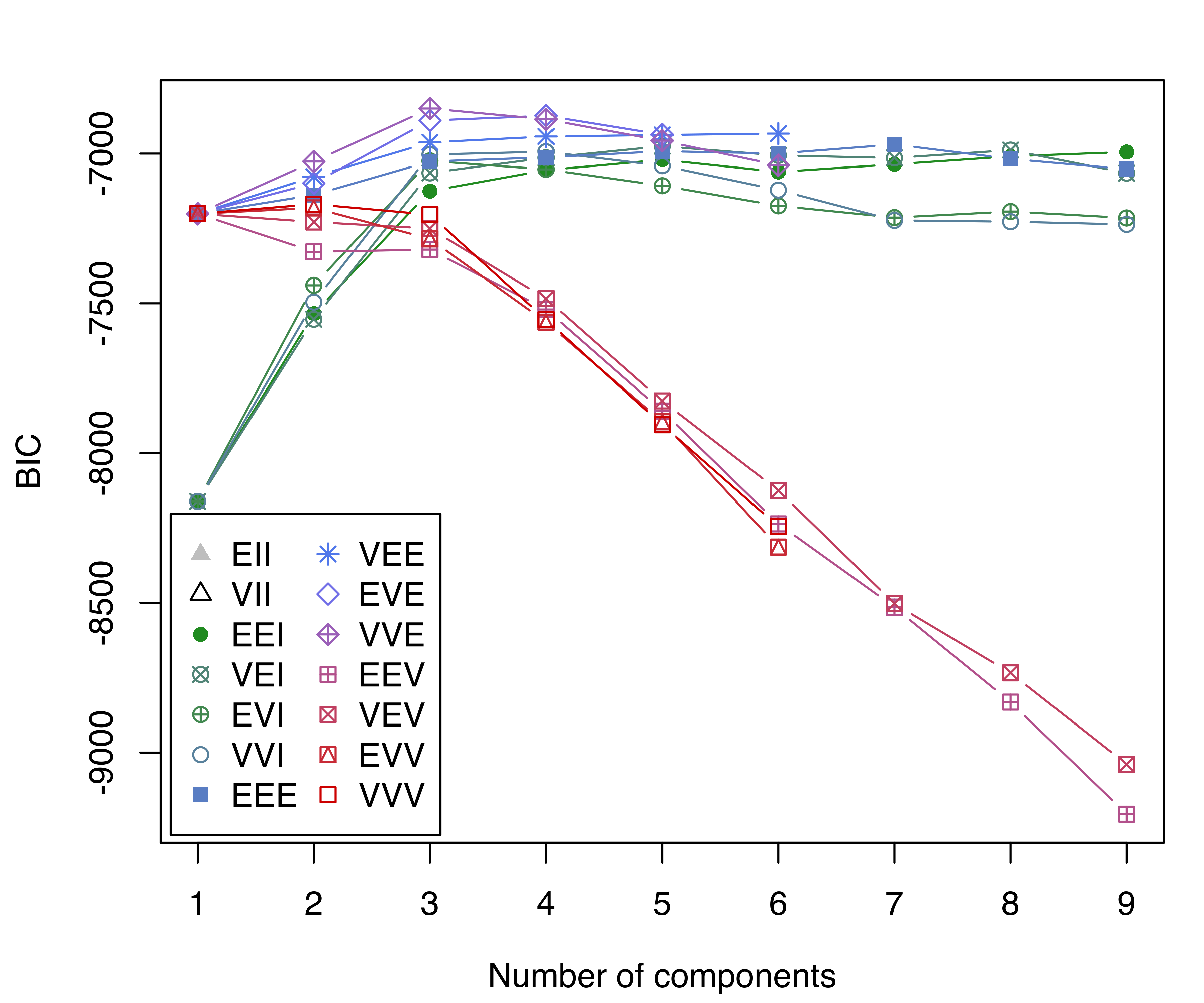
wine data.
Note that, in this last plot, we adjusted the range of the vertical axis so as to remove models with lower BIC values. The model selected by BIC is a three-component Gaussian mixture with covariances having different volumes and shapes, but the same orientation (VVE). This is a flexible but relatively parsimonious model. A summary of the selected model is then obtained:
summary(mod)
## ----------------------------------------------------
## Gaussian finite mixture model fitted by EM algorithm
## ----------------------------------------------------
##
## Mclust VVE (ellipsoidal, equal orientation) model with 3 components:
##
##  log-likelihood   n  df     BIC     ICL
##         -3015.3 178 158 -6849.4 -6850.7
##
## Clustering table:
##  1  2  3
## 59 69 50
table(Class, mod$classification)
##
## Class         1  2  3
##   Barolo     59  0  0
##   Grignolino  0 69  2
##   Barbera     0  0 48
adjustedRandIndex(Class, mod$classification)
## [1] 0.96674
The fitted model provides an accurate recovery of the true classes with a high ARI.
Displaying the results is difficult because of the high dimensionality of the data. Below we give a simple method for choosing a subset of variables for a matrix of scatterplots. More sophisticated approaches to choosing projections that reveal clustering are discussed in Section 6.4. First we plot the estimated cluster means, normalized to the \([0,1]\) range, using the heatmap function available in base R:
norm01 = function(x) (x - min(x))/(max(x) - min(x))
M = apply(t(mod$parameters$mean), 2, norm01)
heatmap(M, Rowv = NA, scale = "none", margins = c(8, 2),
        labRow = paste("Cluster", 1:mod$G), cexRow = 1.2)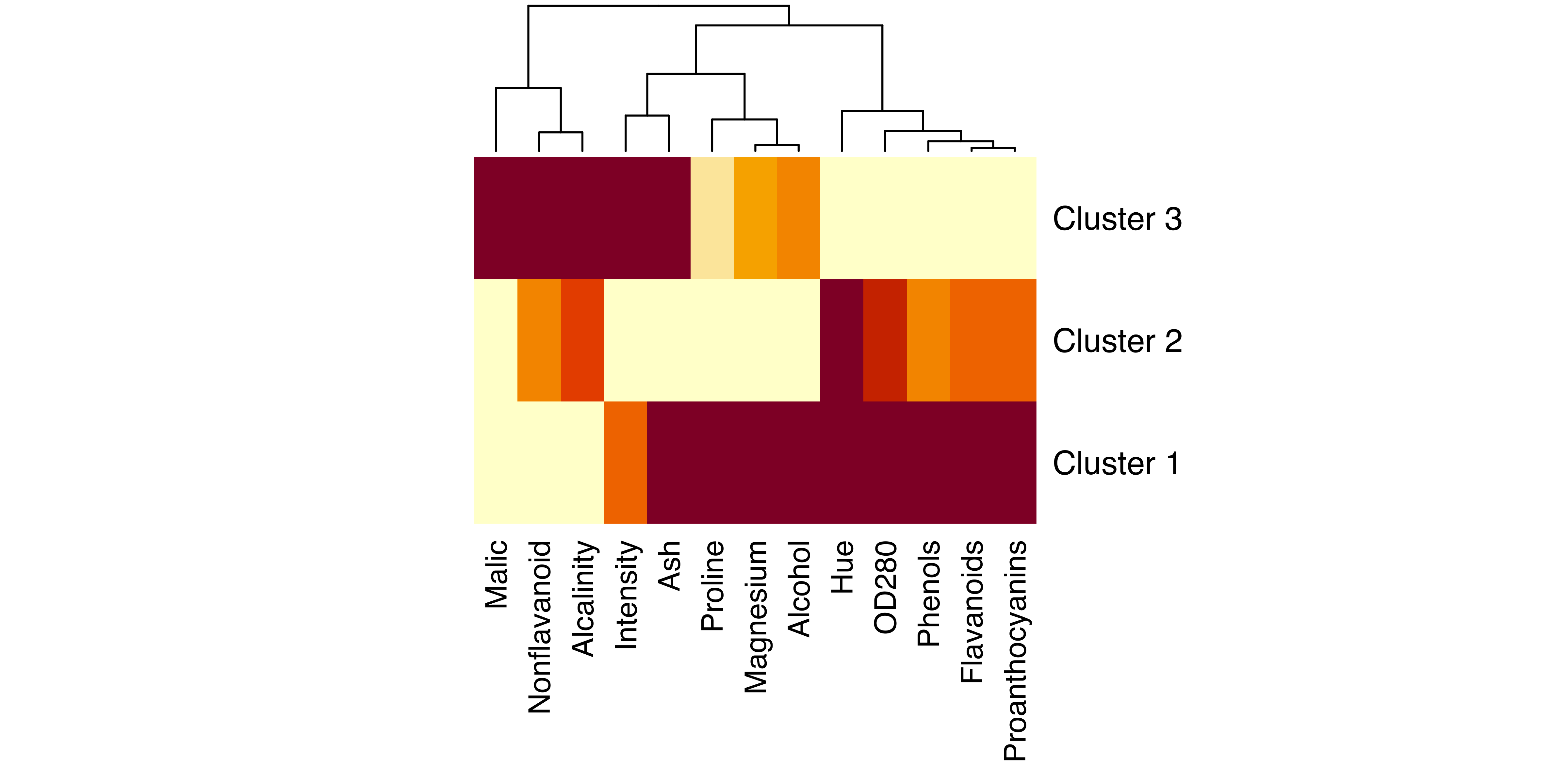
wine data.
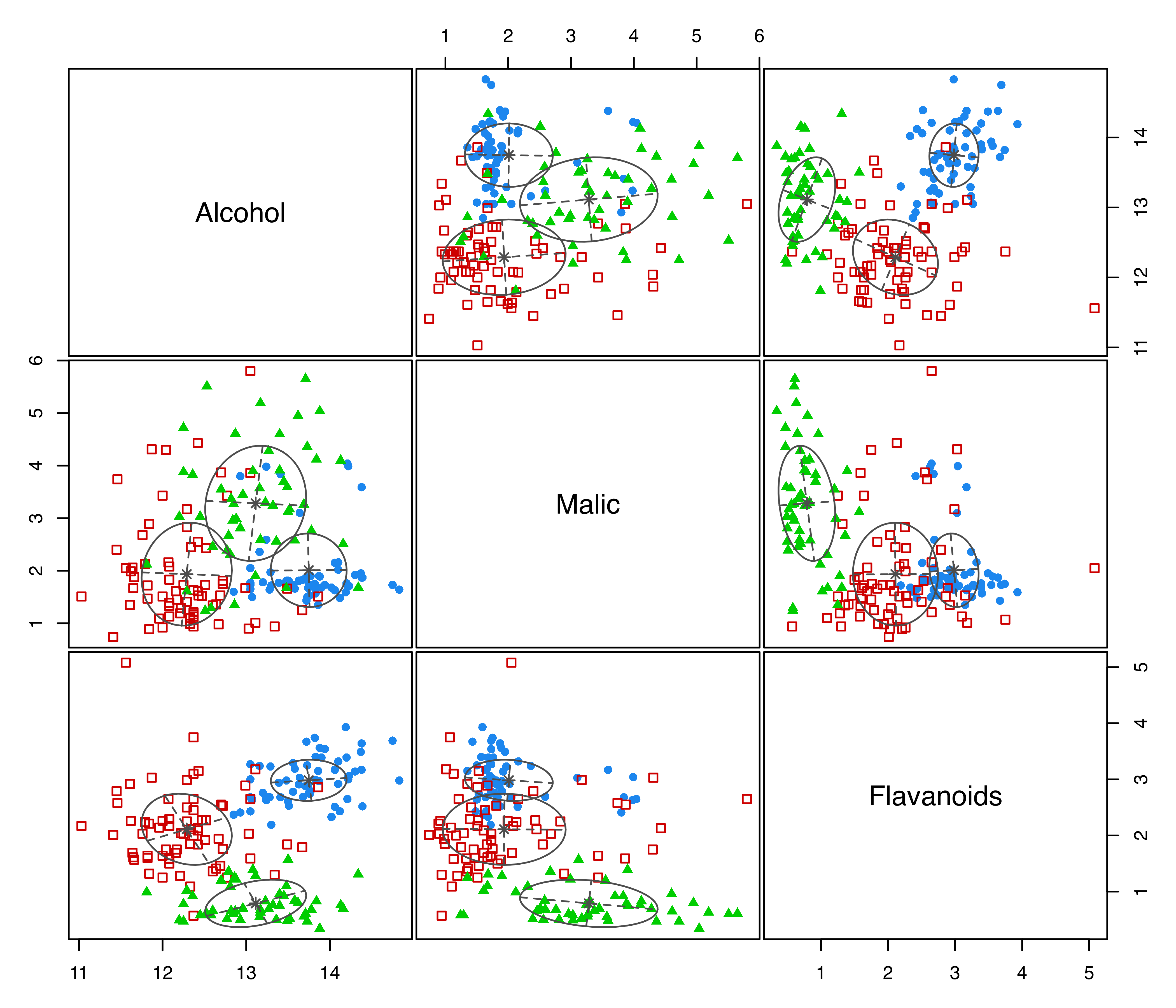
The resulting heatmap (see Figure 3.11) shows which features have the most different cluster means. Based on this, we select a subset of three variables (Alcohol, Malic, and Flavanoids) for the dimens argument specifying coordinate projections for multivariate data in the plot() function call:
3.3 Model Selection
3.3.1 BIC
In the mclust package, BIC is used by default for model selection. The function mclustBIC(), and indirectly Mclust(), computes a matrix of BIC values for models chosen from Table 3.1, and numbers of mixture components as specified.
Example 3.4 BIC model selection for the Old Faithful data
As an illustration, consider the bivariate faithful dataset (Härdle 1991), included in the base R package datasets. “Old Faithful” is a geyser located in Yellowstone National Park, Wyoming, USA. The faithful dataset provides the duration of Old Faithful’s eruptions (eruptions, time in minutes) and the waiting times between successive eruptions (waiting, time in minutes). A scatterplot of the data is shown in panel Figure 3.13, obtained using the code:
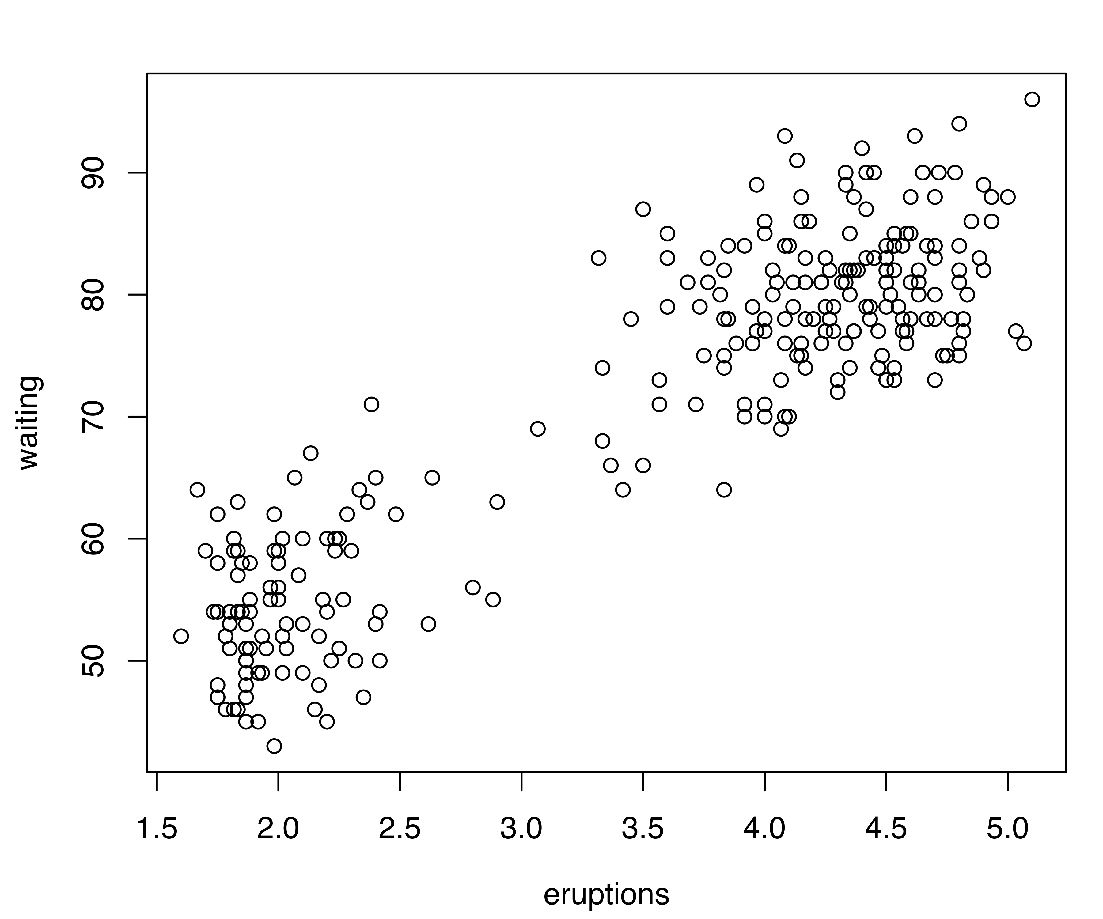
faithful dataset.
The following code can be used to compute the BIC values and plot the corresponding BIC traces:
BIC = mclustBIC(faithful)
BIC
## Bayesian Information Criterion (BIC):
##       EII     VII     EEI     VEI     EVI     VVI     EEE     VEE
## 1 -4024.7 -4024.7 -3055.8 -3055.8 -3055.8 -3055.8 -2607.6 -2607.6
## 2 -3453.0 -3458.3 -2354.6 -2350.6 -2352.6 -2346.1 -2325.2 -2323.0
## 3 -3377.7 -3336.6 -2323.0 -2332.7 -2332.2 -2342.4 -2314.3 -2322.1
## 4 -3230.3 -3242.8 -2323.7 -2331.3 -2334.7 -2343.5 -2331.2 -2340.2
## 5 -3149.4 -3129.1 -2327.1 -2350.2 -2347.6 -2351.0 -2360.7 -2347.3
## 6 -3081.4 -3038.2 -2338.2 -2360.6 -2357.7 -2373.5 -2347.4 -2372.3
## 7 -2990.4 -2973.4 -2356.5 -2368.5 -2372.9 -2394.7 -2369.3 -2371.2
## 8 -2978.1 -2935.1 -2364.1 -2384.7 -2389.1 -2413.7 -2376.1 -2390.4
## 9 -2953.4 -2919.4 -2372.8 -2398.2 -2407.2 -2432.7 -2389.6 -2406.7
##       EVE     VVE     EEV     VEV     EVV     VVV
## 1 -2607.6 -2607.6 -2607.6 -2607.6 -2607.6 -2607.6
## 2 -2324.3 -2320.4 -2329.1 -2325.4 -2327.6 -2322.2
## 3 -2342.3 -2336.3 -2325.3 -2329.6 -2340.0 -2349.7
## 4 -2361.8 -2362.5 -2351.5 -2361.1 -2344.7 -2351.5
## 5 -2351.8 -2368.9 -2356.9 -2368.1 -2364.9 -2379.4
## 6 -2366.5 -2386.5 -2366.1 -2386.3 -2384.1 -2387.0
## 7 -2379.8 -2402.2 -2379.1 -2401.3 -2398.7 -2412.4
## 8 -2403.9 -2426.0 -2393.0 -2425.4 -2415.0 -2442.0
## 9 -2414.1 -2448.2 -2407.5 -2446.7 -2438.9 -2460.4
##
## Top 3 models based on the BIC criterion:
##   EEE,3   VVE,2   VEE,3
## -2314.3 -2320.4 -2322.1
plot(BIC)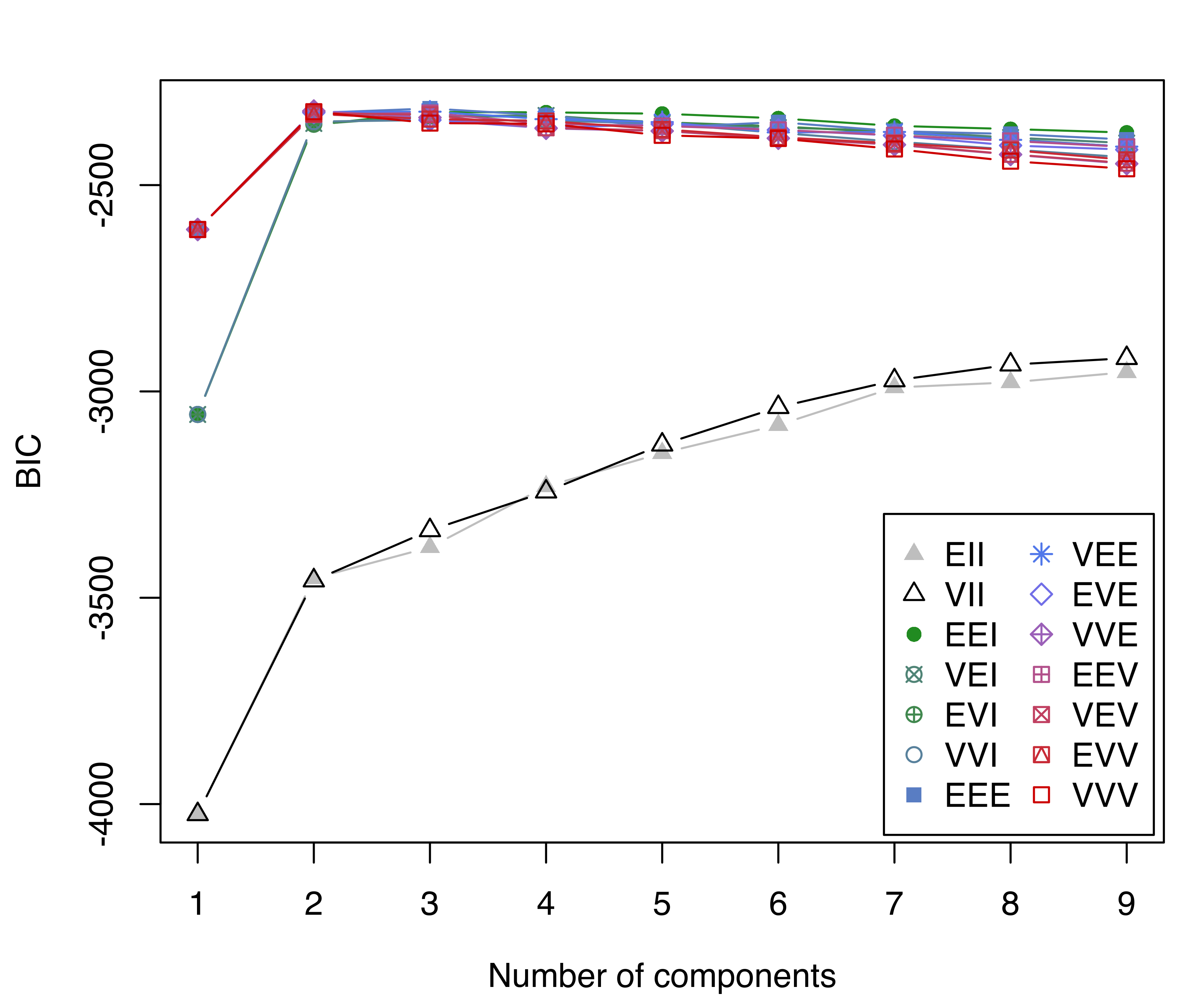
faithful dataset.
In this case the BIC supports a three-component GMM with common full covariance matrix (EEE model). Note that, as for the thyroid disease data example, there are missing BIC values (denoted by NA) corresponding to models that could not be estimated as initialized.
By default, mclustBIC computes results for up to 9 components and all available models in Table 3.1. Optional arguments can be provided to mclustBIC() allowing fine tuning, such as G for the number of components, and modelNames for specifying the model covariance parameterizations (see Table 3.1 and help("mclustModelNames") for a description of available model names).
Another optional argument, called x, can be used to provide the output from a previous call to mclustBIC(). This is useful if the model space needs to be enlarged by fitting more models (by increasing the number of mixture components and/or specifying additional covariance parameterizations) without the need to recompute the BIC values for those models already fitted. BIC values already available can be provided analogously to Mclust as follows:
mod1 = Mclust(faithful, x = BIC)3.3.2 ICL
Besides the BIC criterion for model selection, the integrated complete-data likelihood (ICL) criterion, described in Section 2.3.1, is available in mclust through the function mclustICL(). It is invoked similarly to mclustBIC(), and it allows us to select both the model (among those in Table 3.1) and the number of mixture components that maximize the ICL criterion.
Example 3.5 ICL model selection for the Old Faithful data
Considering again the data in Example 3.4, ICL values are computed as follows:
ICL = mclustICL(faithful)
ICL
## Integrated Complete-data Likelihood (ICL) criterion:
##       EII     VII     EEI     VEI     EVI     VVI     EEE     VEE
## 1 -4024.7 -4024.7 -3055.8 -3055.8 -3055.8 -3055.8 -2607.6 -2607.6
## 2 -3455.8 -3460.9 -2356.3 -2350.7 -2353.3 -2346.2 -2326.7 -2323.4
## 3 -3422.8 -3360.3 -2359.5 -2377.3 -2367.5 -2387.7 -2357.8 -2376.5
## 4 -3265.8 -3272.5 -2372.0 -2413.4 -2402.2 -2436.3 -2468.3 -2452.7
## 5 -3190.7 -3151.9 -2394.0 -2486.7 -2412.4 -2445.8 -2478.2 -2472.0
## 6 -3117.4 -3061.3 -2423.0 -2486.8 -2446.9 -2472.6 -2456.2 -2503.9
## 7 -3022.3 -2995.8 -2476.2 -2519.8 -2446.7 -2496.7 -2464.3 -2466.8
## 8 -3007.4 -2953.7 -2488.5 -2513.5 -2492.3 -2509.7 -2502.2 -2479.8
## 9 -2989.1 -2933.1 -2499.9 -2540.4 -2515.0 -2528.6 -2547.1 -2499.9
##       EVE     VVE     EEV     VEV     EVV     VVV
## 1 -2607.6 -2607.6 -2607.6 -2607.6 -2607.6 -2607.6
## 2 -2325.8 -2320.8 -2330.0 -2325.7 -2328.2 -2322.7
## 3 -2412.0 -2427.0 -2372.4 -2405.3 -2380.3 -2385.2
## 4 -2459.4 -2440.3 -2414.2 -2419.9 -2385.8 -2407.6
## 5 -2444.3 -2478.6 -2431.1 -2490.2 -2423.2 -2474.5
## 6 -2504.8 -2489.1 -2449.6 -2481.4 -2483.8 -2491.6
## 7 -2499.3 -2496.3 -2465.7 -2506.8 -2490.1 -2519.5
## 8 -2526.0 -2516.6 -2489.4 -2539.8 -2497.8 -2556.1
## 9 -2545.7 -2541.7 -2542.9 -2566.7 -2528.6 -2587.2
##
## Top 3 models based on the ICL criterion:
##   VVE,2   VVV,2   VEE,2
## -2320.8 -2322.7 -2323.4
A trace of ICL values is plotted and shown in Figure 3.15:
plot(ICL)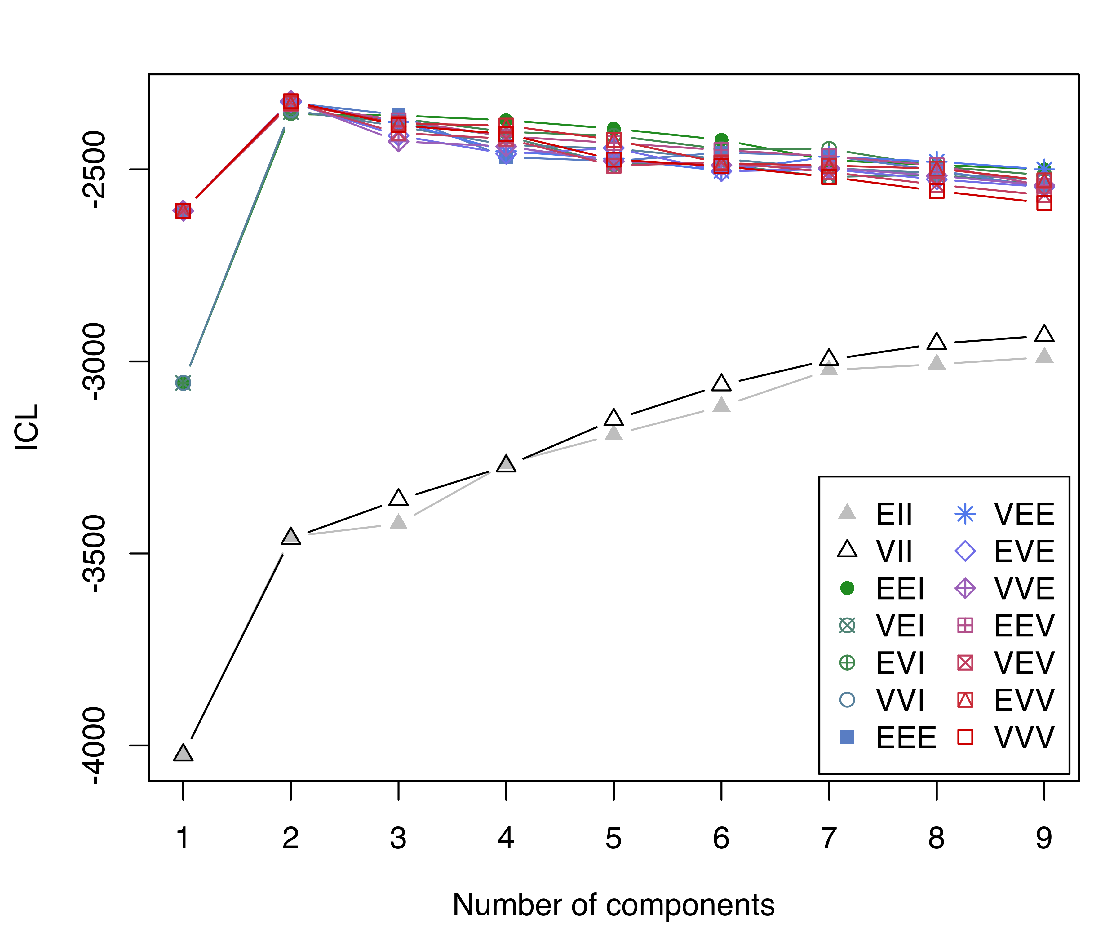
faithful dataset.
Note that, in this case, ICL selects two components, one less than the number selected by BIC. This is reasonable, since ICL penalizes overlapping components more heavily.
The model selected by ICL can be fitted using
mod2 = Mclust(faithful, G = 2, modelNames = "VVE")Optional arguments can also be provided in the Mclust() function call, analogous to those described above for mclustBIC().
The following code can be used to draw scatterplots of the data with points marked according to the classification obtained by the ``best’’ estimated model selected, respectively, by the BIC and ICL model selection criteria (see Figure 3.16):
plot(mod1, what = "classification", fillEllipses = TRUE)
plot(mod2, what = "classification", fillEllipses = TRUE)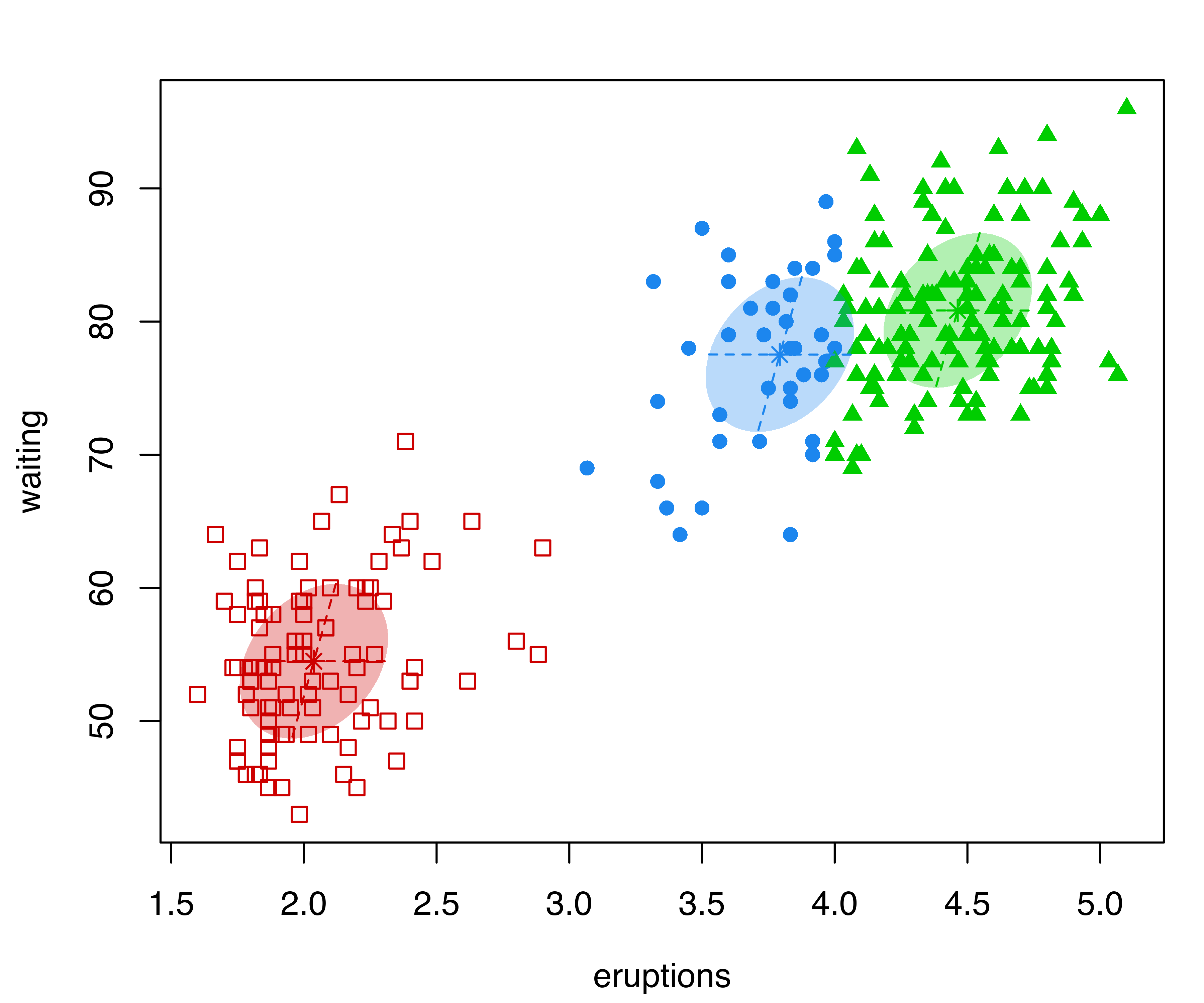
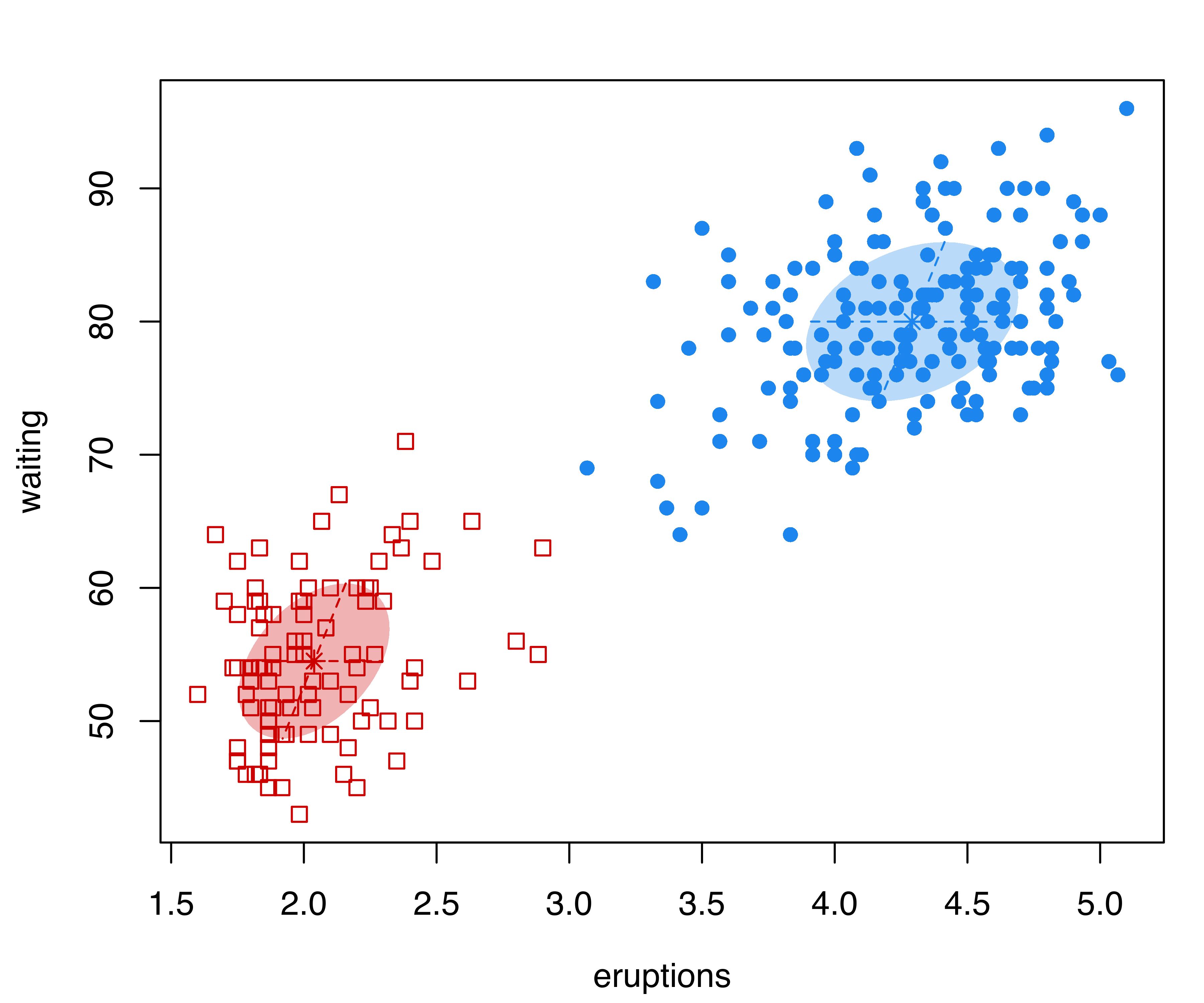
faithful dataset with points and ellipses corresponding to the classification from the best estimated GMMs selected by BIC (a) and ICL (b).
3.3.3 Bootstrap Likelihood Ratio Testing
The bootstrap procedure discussed in Section 2.3.2 for selecting the number of mixture components is implemented in the mclustBootstrapLRT() function.
Example 3.6 Bootstrap LRT for the Old Faithful data
Using the data of {Example 3.4}, a bootstrap LR test is obtained by specifying the input data and the name of the model to test:
LRT = mclustBootstrapLRT(faithful, modelName = "VVV")
LRT
## -------------------------------------------------------------
## Bootstrap sequential LRT for the number of mixture components
## -------------------------------------------------------------
## Model        = VVV
## Replications = 999
##              LRTS bootstrap p-value
## 1 vs 2   319.0654             0.001
## 2 vs 3     6.1305             0.572
The sequential bootstrap procedure terminates when a test is not significant as specified by the argument level (which is set to 0.05 by default). There is also the option to specify the maximum number of mixture components to test via the argument maxG. The number of bootstrap resamples can be set with the optional argument nboot (nboot = 999 is the default).
In the example above, the bootstrap \(p\)-values clearly indicate the presence of two clusters. Note that models fitted to the original data are estimated via the EM algorithm initialized with unconstrained model-based agglomerative hierarchical clustering (the default). Then, during the bootstrap procedure, models under the null and the alternative hypotheses are fitted to bootstrap samples using again the EM algorithm. However, in this case the algorithm starts with the E-step initialized with the estimated parameters obtained for the original data.
The bootstrap distributions of the LRTS can be shown graphically (see Figure 3.17) using the associated plot method:
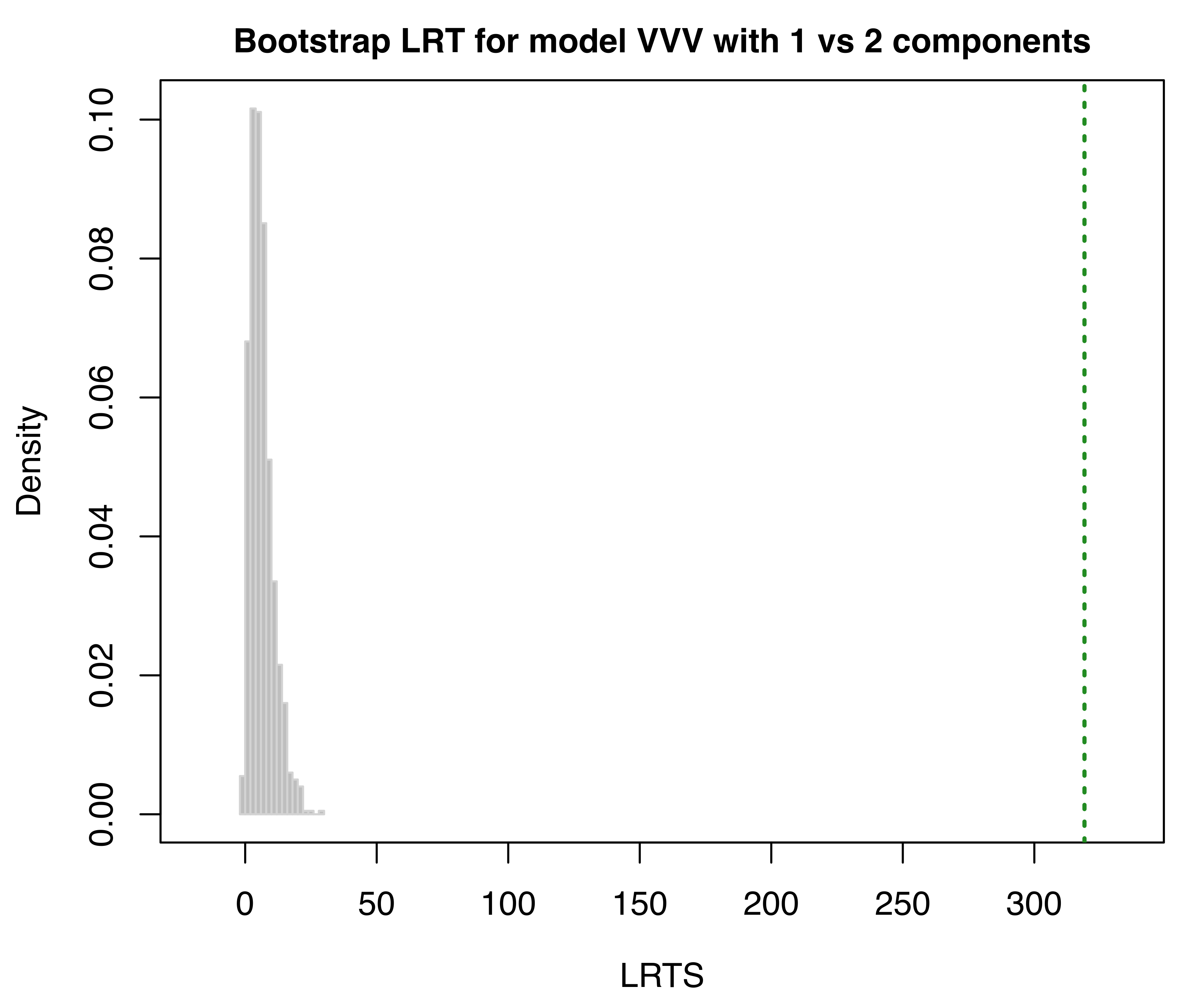
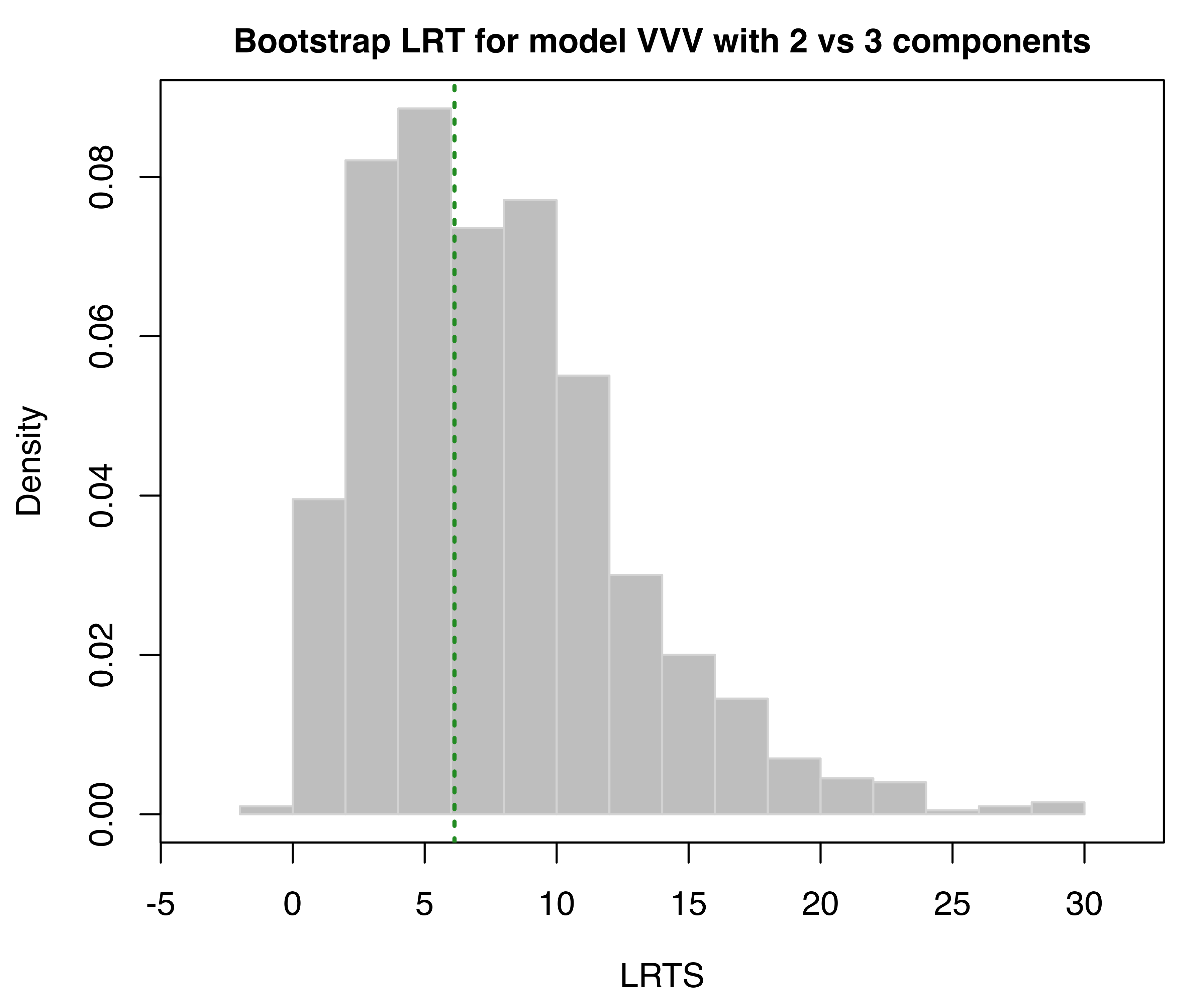
faithful data assuming the VVV model. The dotted vertical lines refer to the sample values of LRTS.
3.4 Resampling-Based Inference in mclust
Section 2.4 describes some resampling-based approaches to inference in GMMs, namely the nonparametric bootstrap, the parametric bootstrap, and the weighted likelihood bootstrap. These, together with the jackknife (Efron 1979, Efron:1982), are implemented in the MclustBootstrap() function available in mclust.
Example 3.7 Resampling-based inference for Gaussian mixtures on the hemophilia data
Consider the hemophilia dataset (Habbema, Hermans, and Broek 1974) available in the package rrcov (Todorov 2022), which contains two measured variables on 75 women belonging to two groups: 30 of them are non-carriers (normal group) and 45 are known hemophilia A carriers (obligatory carriers).
The last command plots the known classification of the observed data (see Figure 3.18 (a)).
By analogy with the analysis of Basford et al. (1997, Example II, Section 5), we fitted a two-component GMM with unconstrained covariance matrices:
mod = Mclust(X, G = 2, modelName = "VVV")
summary(mod, parameters = TRUE)
## ----------------------------------------------------
## Gaussian finite mixture model fitted by EM algorithm
## ----------------------------------------------------
##
## Mclust VVV (ellipsoidal, varying volume, shape, and orientation) model
## with 2 components:
##
##  log-likelihood  n df    BIC    ICL
##          77.029 75 11 106.56 92.855
##
## Clustering table:
##  1  2
## 39 36
##
## Mixing probabilities:
##       1       2
## 0.51015 0.48985
##
## Means:
##                  [,1]      [,2]
## AHFactivity -0.116124 -0.366387
## AHFantigen  -0.024573 -0.045323
##
## Variances:
## [,,1]
##             AHFactivity AHFantigen
## AHFactivity   0.0113599  0.0065959
## AHFantigen    0.0065959  0.0123872
## [,,2]
##             AHFactivity AHFantigen
## AHFactivity    0.015874   0.015050
## AHFantigen     0.015050   0.032341
Note that, in the summary() function call, we set parameters = TRUE to retrieve the estimated parameters. The clustering structure identified is shown in Figure 3.18 (b) and can be obtained as follows:
plot(mod, what = "classification", fillEllipses = TRUE)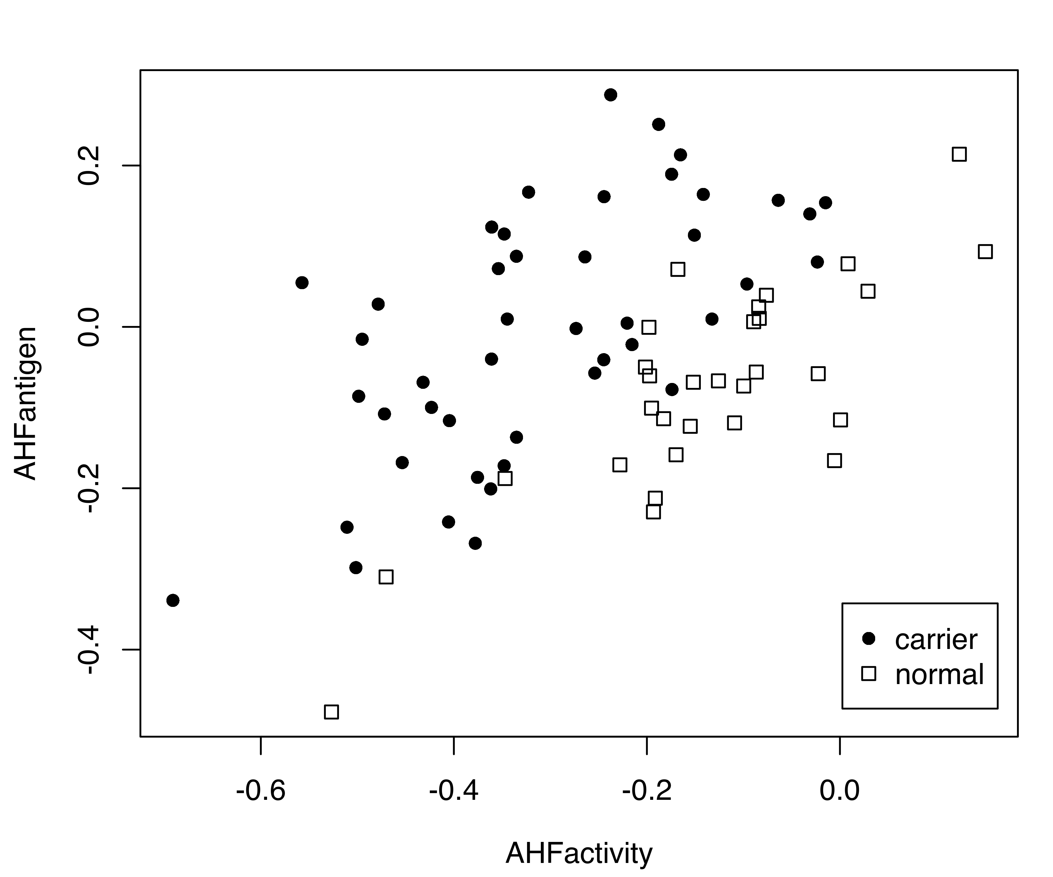
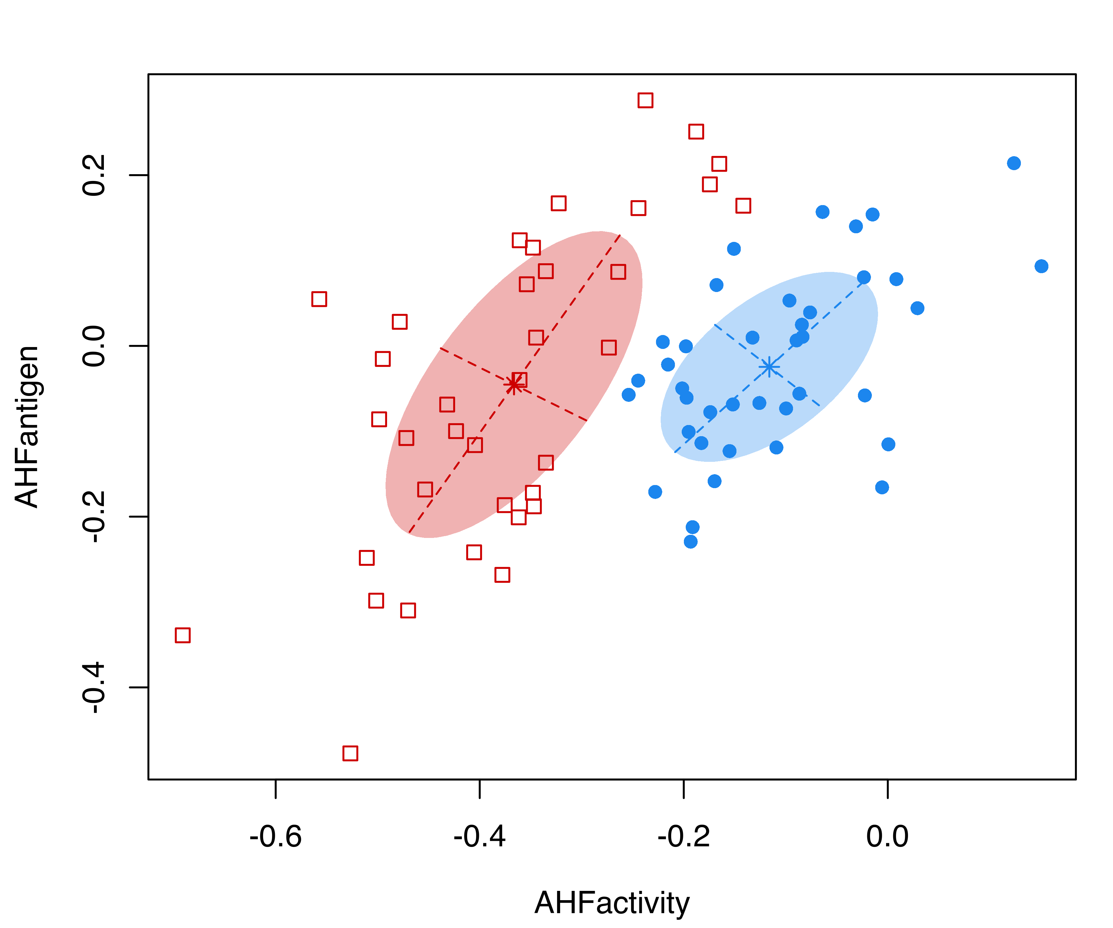
hemophilia data displaying the true class membership (a) and the classification obtained from the fit of a GMM (b).
A function, MclustBootstrap(), is available for bootstrap inference for GMMs. This function requires the user to input an object as returned by a call to Mclust(). Optionally, the number of bootstrap resamples (nboot) and the type of bootstrap resampling to use (type), can also be specified. By default, nboot = 999 and type = "bs", with the latter specifying the nonparametric bootstrap. Thus, a simple call for computing the bootstrap distribution of the GMM parameters is the following:
boot = MclustBootstrap(mod, nboot = 999, type = "bs")Note that, although we have included the arguments nboot and type, they could have been omitted in this instance since they are both set at their defaults.
Results of the function MclustBootstrap() are available through the summary() method, which by default returns the standard errors of the GMM parameters:
summary(boot, what = "se")
## ----------------------------------------------------------
## Resampling standard errors
## ----------------------------------------------------------
## Model                      = VVV
## Num. of mixture components = 2
## Replications               = 999
## Type                       = nonparametric bootstrap
##
## Mixing probabilities:
##       1       2
## 0.12032 0.12032
##
## Means:
##                    1        2
## AHFactivity 0.037581 0.041488
## AHFantigen  0.030828 0.062937
##
## Variances:
## [,,1]
##             AHFactivity AHFantigen
## AHFactivity   0.0065336  0.0044027
## AHFantigen    0.0044027  0.0030834
## [,,2]
##             AHFactivity AHFantigen
## AHFactivity   0.0062451  0.0056968
## AHFantigen    0.0056968  0.0093190
Bootstrap percentile confidence intervals, described in Section 2.4, can also be obtained by specifying what = "ci" in the summary() call. The confidence level of the intervals can also be specified (by default, conf.level = 0.95). For instance:
summary(boot, what = "ci", conf.level = 0.9)
## ----------------------------------------------------------
## Resampling confidence intervals
## ----------------------------------------------------------
## Model                      = VVV
## Num. of mixture components = 2
## Replications               = 999
## Type                       = nonparametric bootstrap
## Confidence level           = 0.9
##
## Mixing probabilities:
##           1       2
## 5%  0.37514 0.22068
## 95% 0.77932 0.62486
##
## Means:
## [,,1]
##     AHFactivity AHFantigen
## 5%     -0.20610  -0.079998
## 95%    -0.08424   0.020474
## [,,2]
##     AHFactivity AHFantigen
## 5%     -0.43889  -0.132681
## 95%    -0.30504   0.097313
##
## Variances:
## [,,1]
##     AHFactivity AHFantigen
## 5%    0.0056903  0.0081596
## 95%   0.0265706  0.0181777
## [,,2]
##     AHFactivity AHFantigen
## 5%    0.0050765  0.0096963
## 95%   0.0247648  0.0423184
The bootstrap distribution of the parameters can also be represented graphically. For instance, the following code produces a plot of the bootstrap distribution for the mixing proportions:
plot(boot, what = "pro")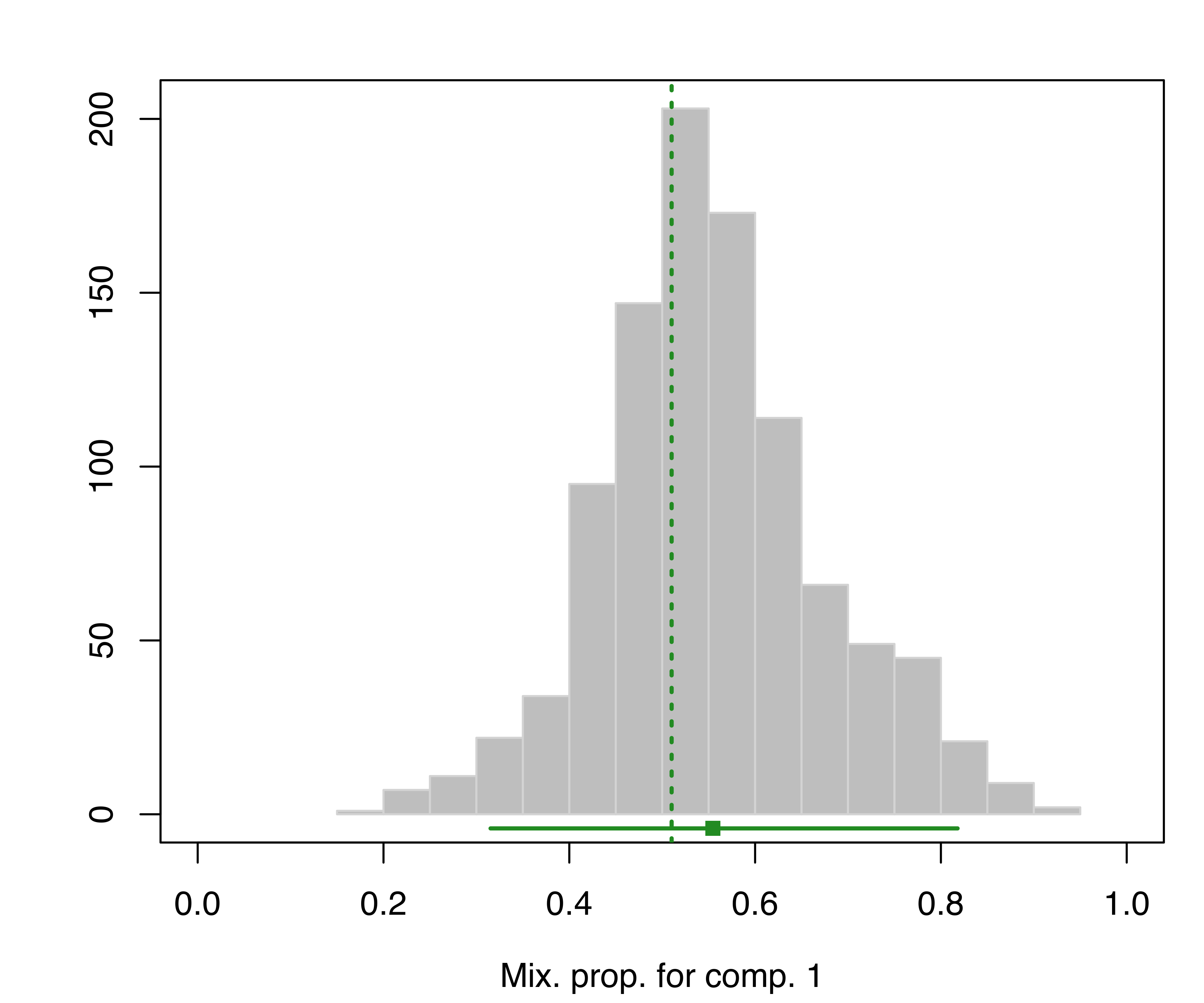
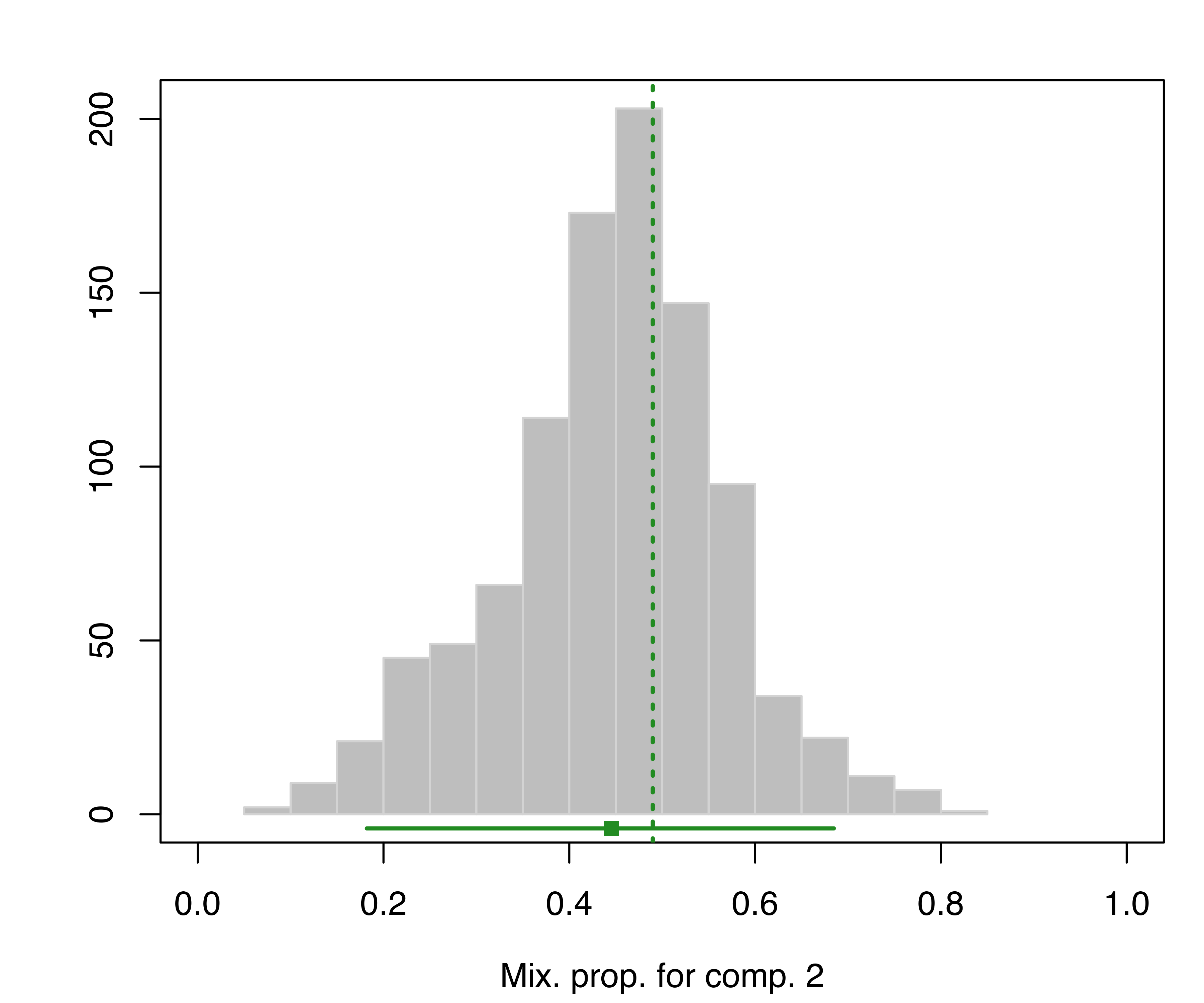
hemophilia data. The vertical dotted lines indicate the MLEs, the bottom line indicates the percentile confidence intervals, and the square shows the center of the bootstrap distribution.
and for the component means:
plot(boot, what = "mean")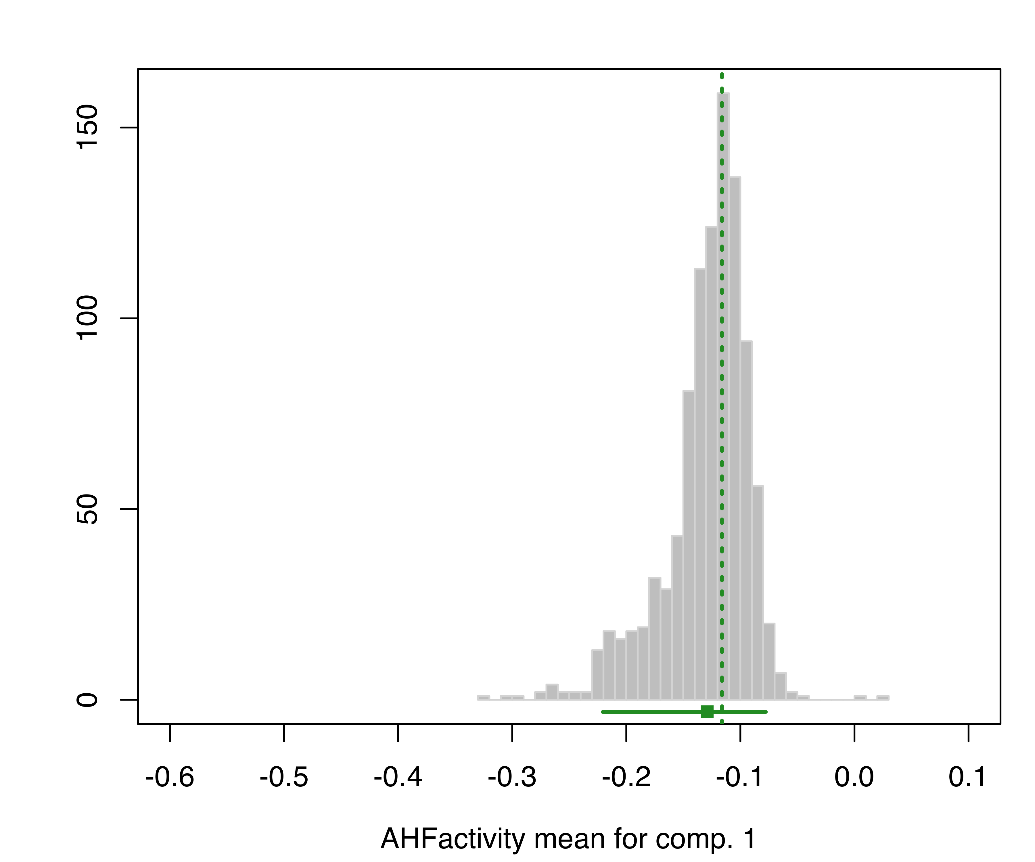
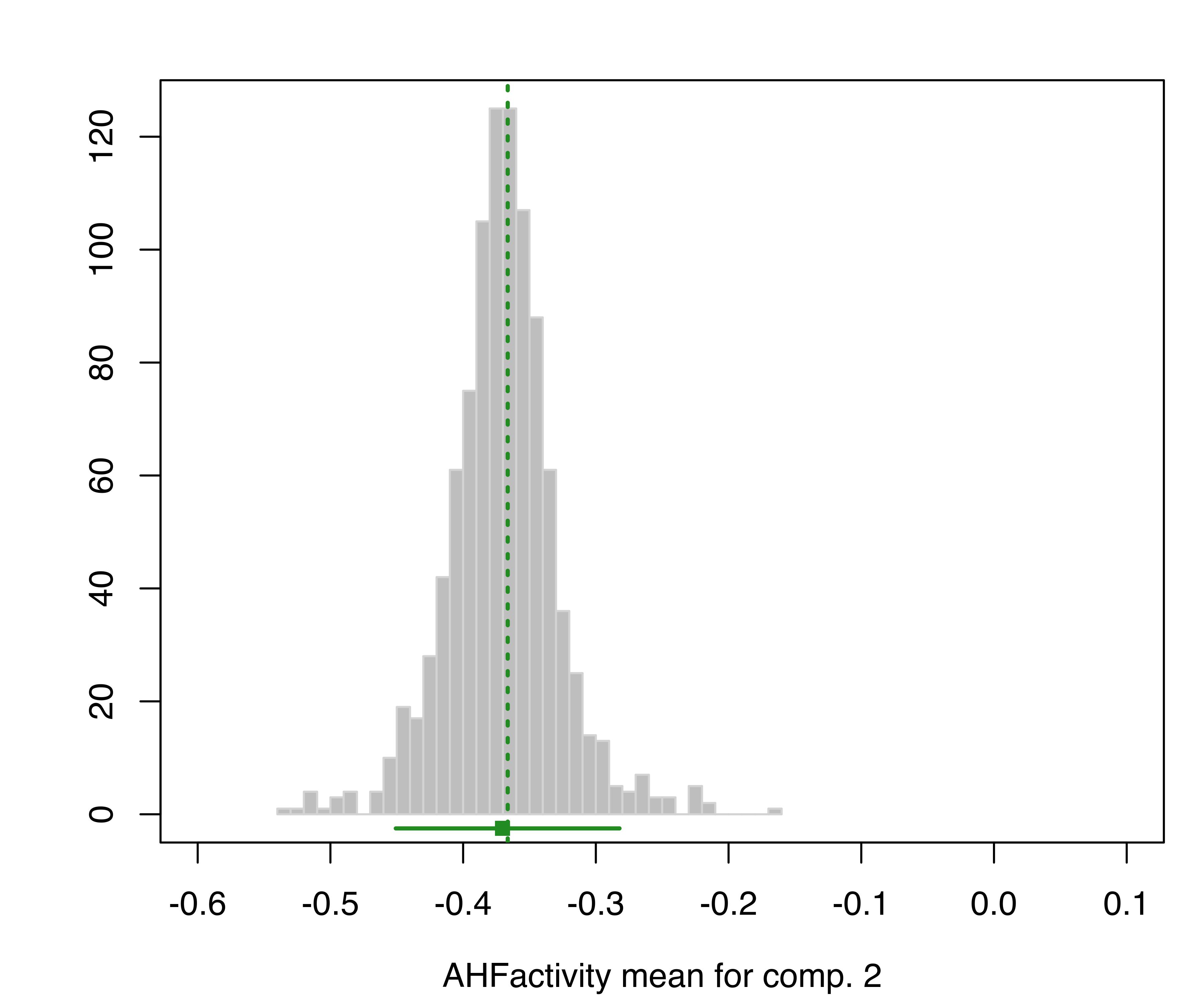
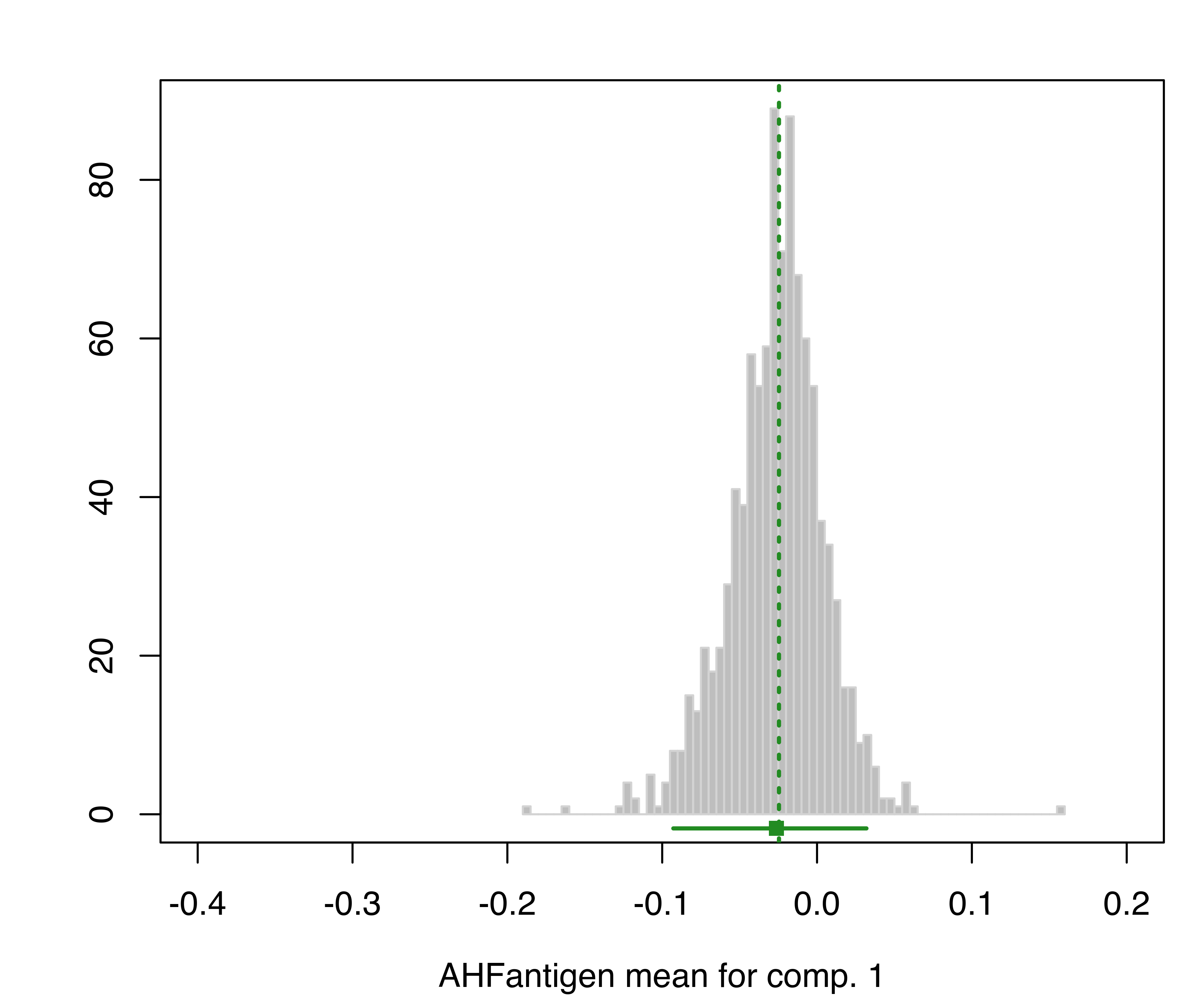
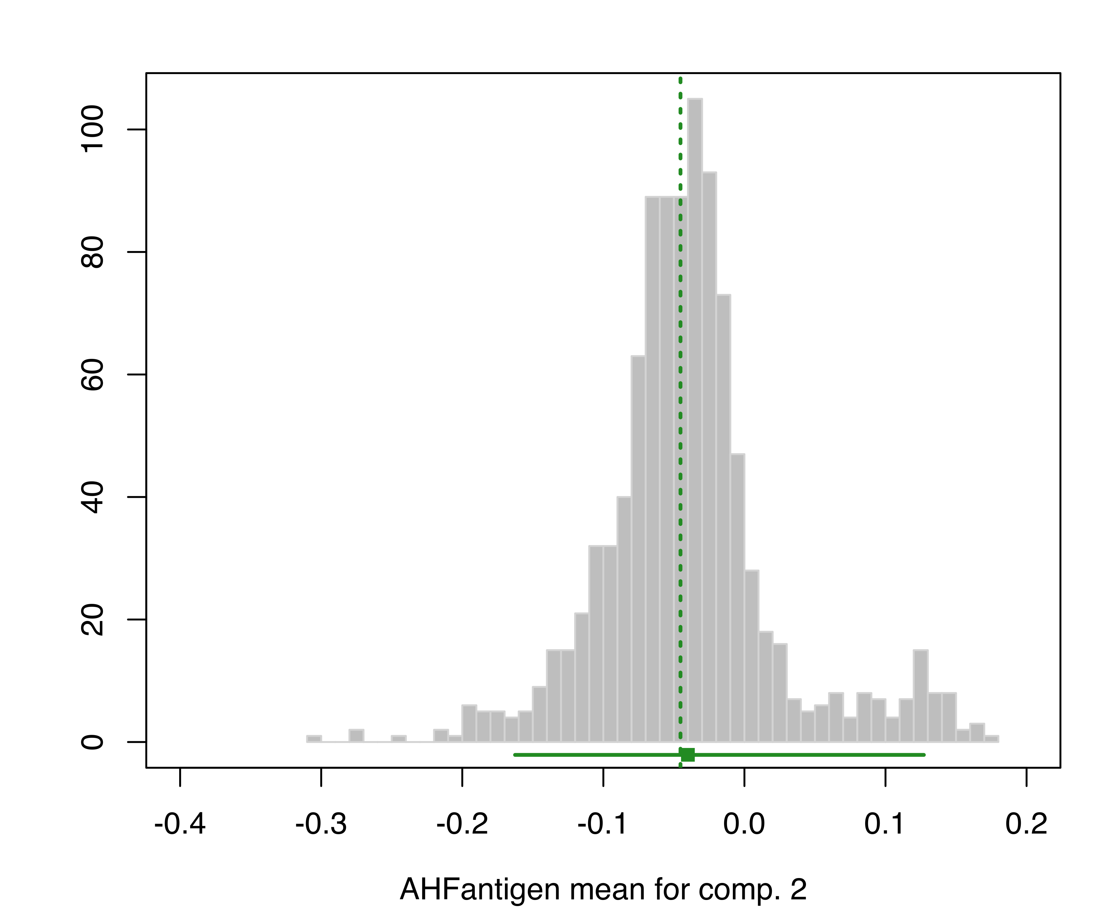
hemophilia data. The vertical dotted lines indicate the MLEs, the bottom line indicates the percentile confidence intervals, and the square shows the center of the bootstrap distribution.
The resulting plots are shown in Figure 3.19 and Figure 3.20.
As mentioned, with the function MclustBootstrap(), it is also possible to choose the parametric bootstrap (type = "pb"), the weighted likelihood bootstrap (type = "wlbs"), or the jackknife (type = "jk"). For instance, in our data example the weighted likelihood bootstrap can be obtained as follows:
wlboot = MclustBootstrap(mod, nboot = 999, type = "wlbs")
summary(wlboot, what = "se")
## ----------------------------------------------------------
## Resampling standard errors
## ----------------------------------------------------------
## Model                      = VVV
## Num. of mixture components = 2
## Replications               = 999
## Type                       = weighted likelihood bootstrap
##
## Mixing probabilities:
##       1       2
## 0.12062 0.12062
##
## Means:
##                    1        2
## AHFactivity 0.037307 0.040271
## AHFantigen  0.029360 0.064102
##
## Variances:
## [,,1]
##             AHFactivity AHFantigen
## AHFactivity   0.0063976  0.0042667
## AHFantigen    0.0042667  0.0029802
## [,,2]
##             AHFactivity AHFantigen
## AHFactivity   0.0056345  0.0057299
## AHFantigen    0.0057299  0.0093274
In this case the differences between the nonparametric and the weighted likelihood bootstrap are negligible. We can summarize the inference for the GMM component means obtained under the two approaches graphically, showing the bootstrap percentile confidence intervals for each variable and component (see Figure 3.21):
boot.ci = summary(boot, what = "ci")
wlboot.ci = summary(wlboot, what = "ci")
for (j in 1:mod$d)
{
  plot(1:mod$G, mod$parameters$mean[j, ], col = 1:mod$G, pch = 15,
       ylab = colnames(X)[j], xlab = "Mixture component",
       ylim = range(boot.ci$mean, wlboot.ci$mean),
       xlim = c(.5, mod$G+.5), xaxt = "n")
  points(1:mod$G+0.2, mod$parameters$mean[j, ], col = 1:mod$G, pch = 15)
  axis(side = 1, at = 1:mod$G)
  with(boot.ci,
       errorBars(1:G, mean[1, j, ], mean[2, j, ], col = 1:G))
  with(wlboot.ci,
       errorBars(1:G+0.2, mean[1, j, ], mean[2, j, ], col = 1:G, lty = 2))
}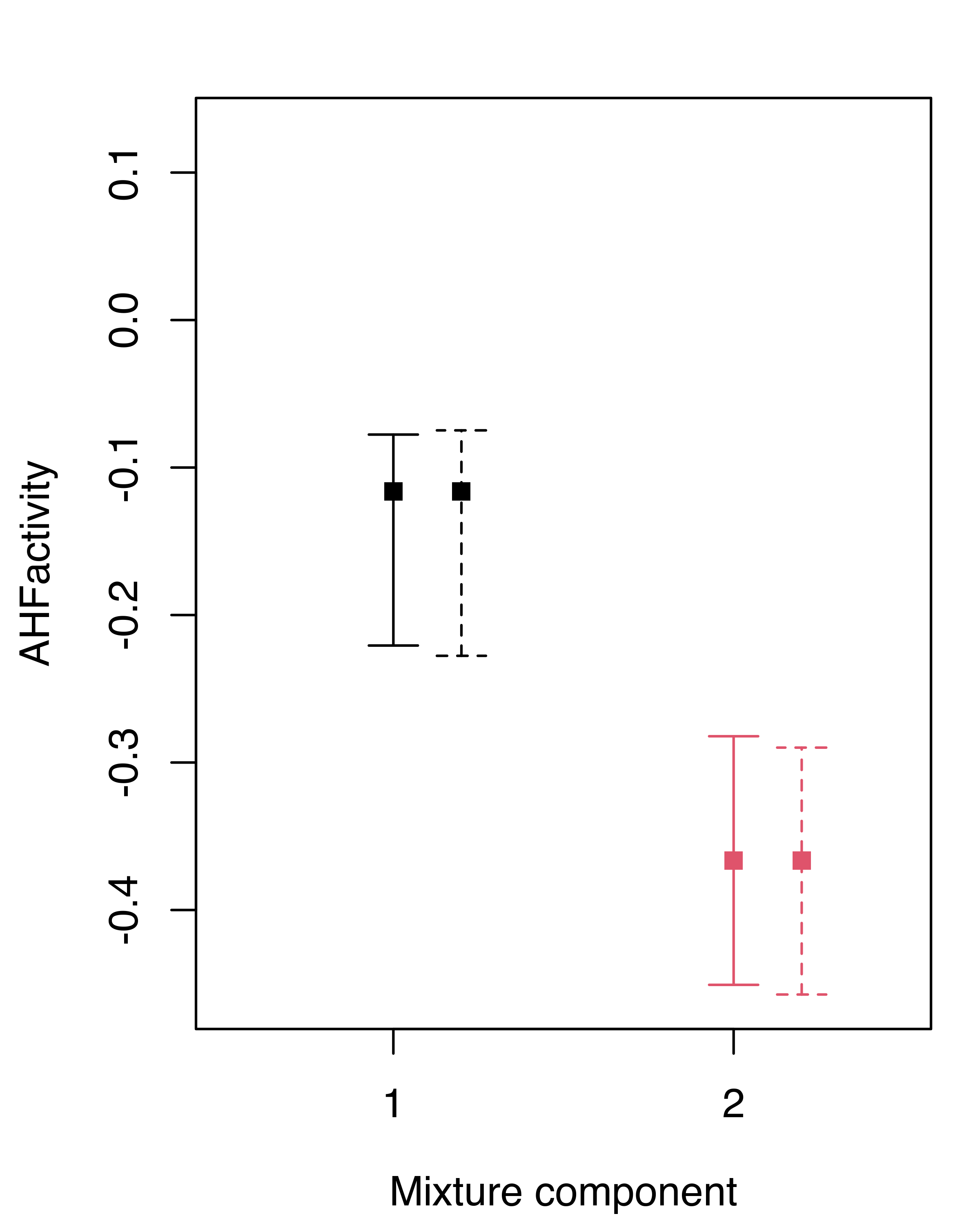
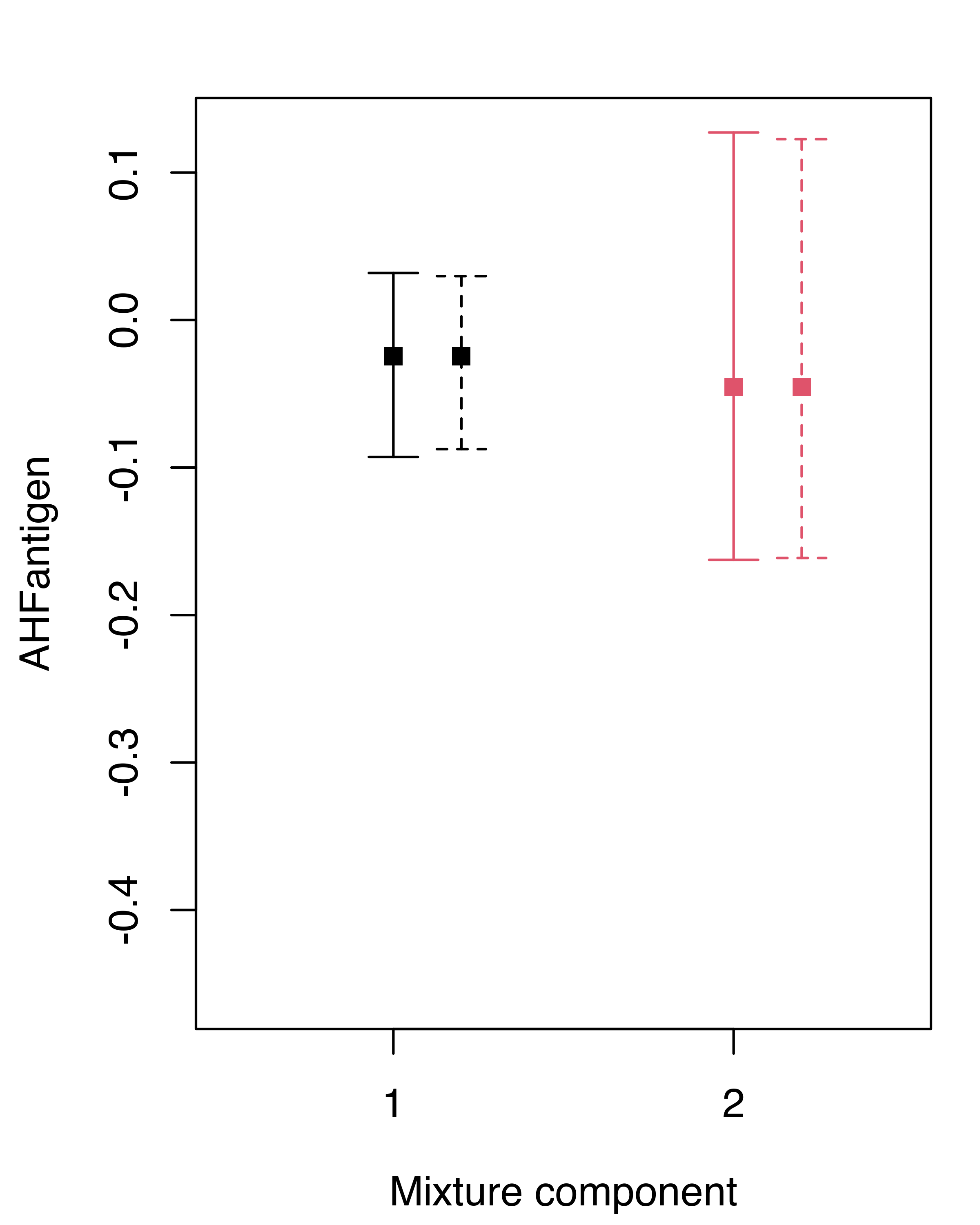
hemophilia data. Solid lines refer to the nonparametric bootstrap, dashed lines to the weighted likelihood bootstrap.
3.5 Clustering Univariate Data
For clustering univariate data, the quantiles of the empirical distribution are used to initialize the EM algorithm by default, rather than hierarchical clustering. There are only two possible models, E for equal variance across components and V allowing the variance to vary across the components.
Example 3.8 Univariate clustering of annual precipitation in US cities
As an example of univariate clustering, consider the precip dataset (McNeil 1977) included in the package datasets available in the base R distribution:
data("precip", package = "datasets")
dotchart(sort(precip), cex = 0.6, pch = 19,
         xlab = "Average annual rainfall (in inches)")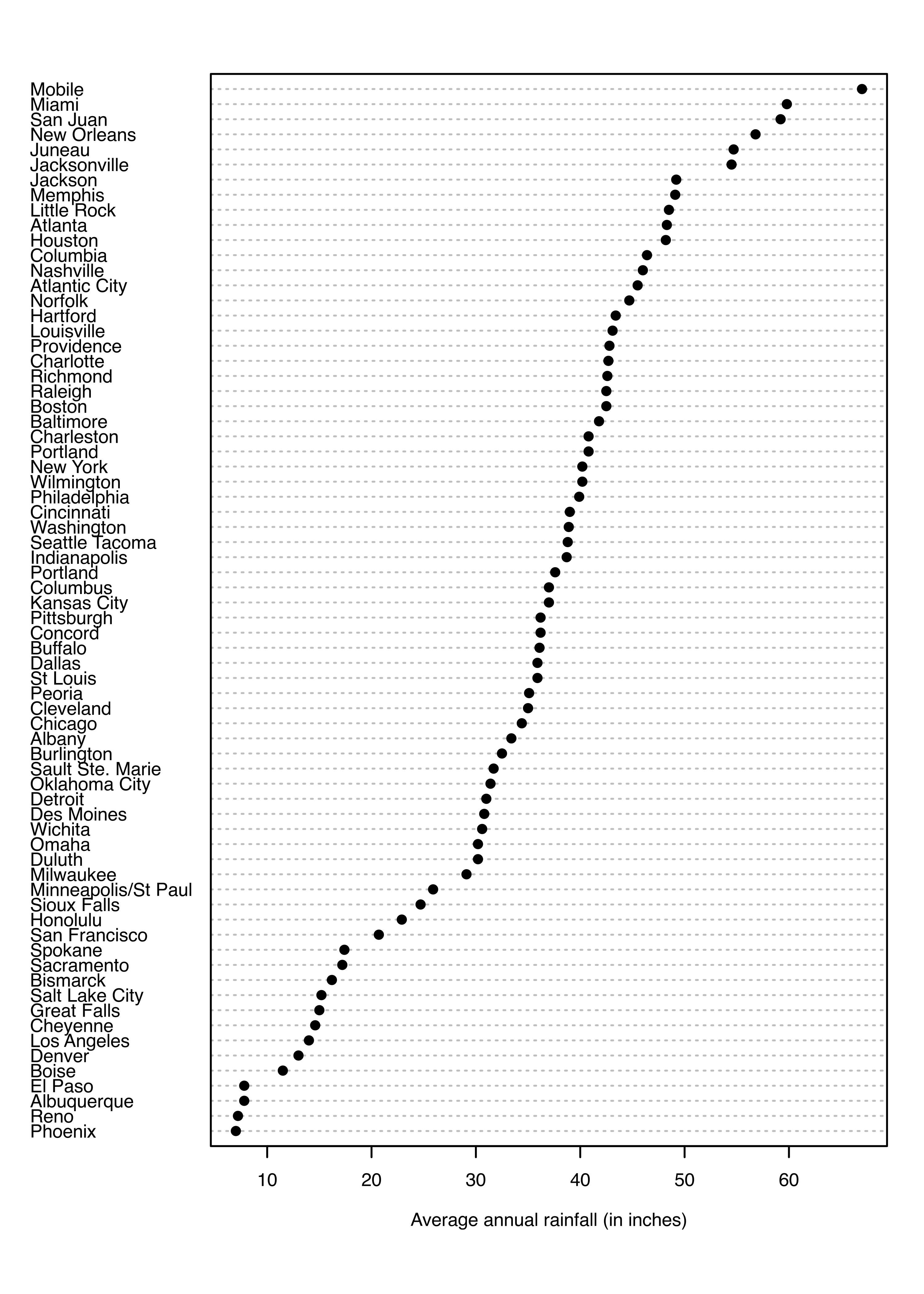
The average amount of rainfall (in inches) for each of 70 US cities is shown as a dot chart in Figure 3.22. A clustering model is then obtained as follows:
mod = Mclust(precip)
summary(mod, parameters = TRUE)
## ----------------------------------------------------
## Gaussian finite mixture model fitted by EM algorithm
## ----------------------------------------------------
##
## Mclust V (univariate, unequal variance) model with 2 components:
##
##  log-likelihood  n df     BIC     ICL
##         -275.47 70  5 -572.19 -575.21
##
## Clustering table:
##  1  2
## 13 57
##
## Mixing probabilities:
##       1       2
## 0.18137 0.81863
##
## Means:
##      1      2
## 12.793 39.780
##
## Variances:
##      1      2
## 16.813 90.394
plot(mod, what = "BIC", legendArgs = list(x = "bottomleft"))
precip data.
The selected model is a two-component Gaussian mixture with different variances. The first cluster, which includes 13 cities, is characterized by both smaller means and variances compared to the second cluster. The clustering partition and the corresponding classification uncertainties can be displayed using the following plot commands (see Figure 3.24):
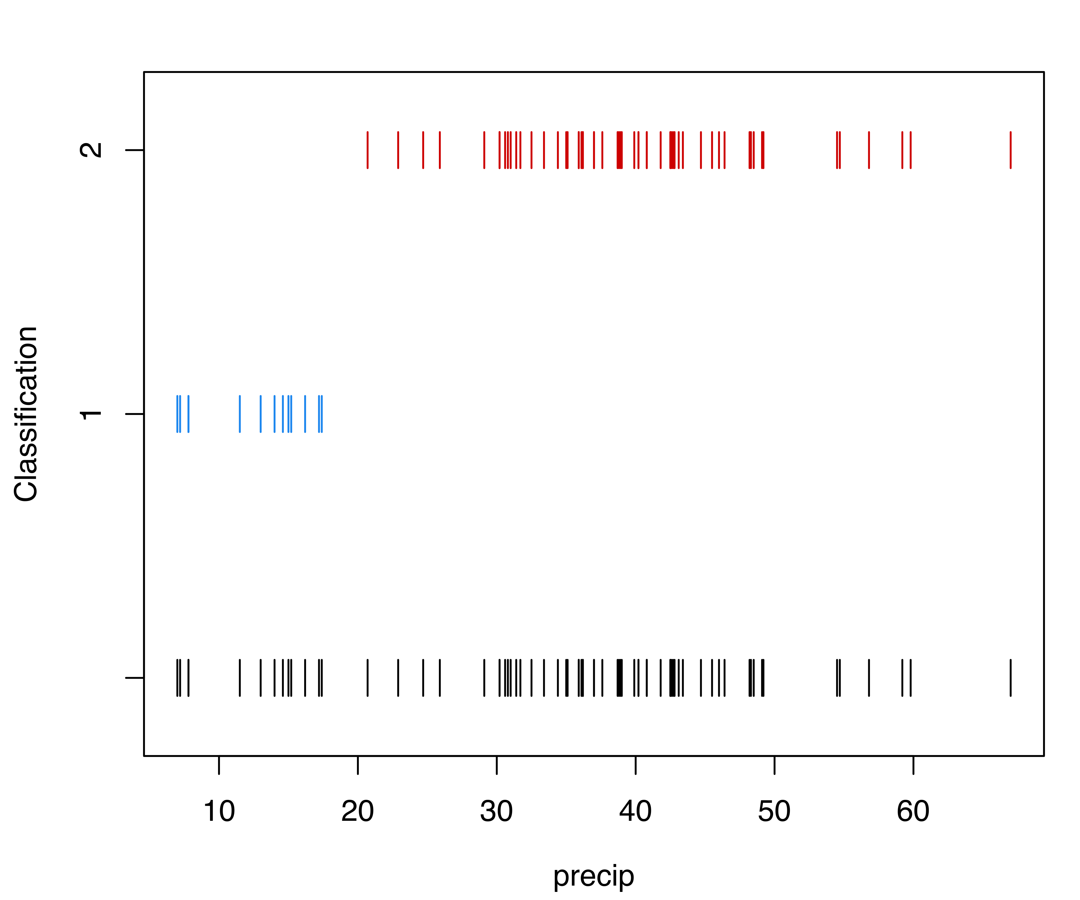
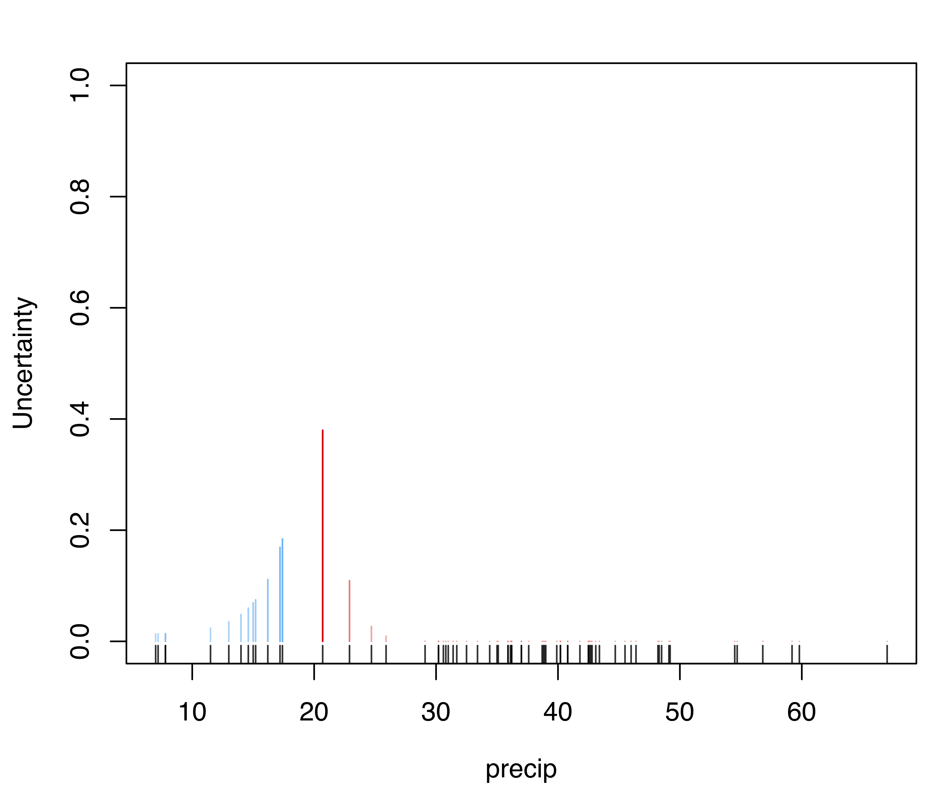
precip data.
The final clustering is shown in a dot chart with observations grouped by clusters (see Figure 3.25):
x = data.frame(precip, clusters = mod$classification)
rownames(x) = make.unique(names(precip)) # correct duplicated names
x = x[order(x$precip), ]
dotchart(x$precip, labels = rownames(x),
         groups = factor(x$clusters, levels = 2:1,
                         labels = c("Cluster 2", "Cluster 1")),
         cex = 0.6, pch = 19,
         color = mclust.options("classPlotColors")[x$clusters],
         xlab = "Average annual rainfall (in inches)")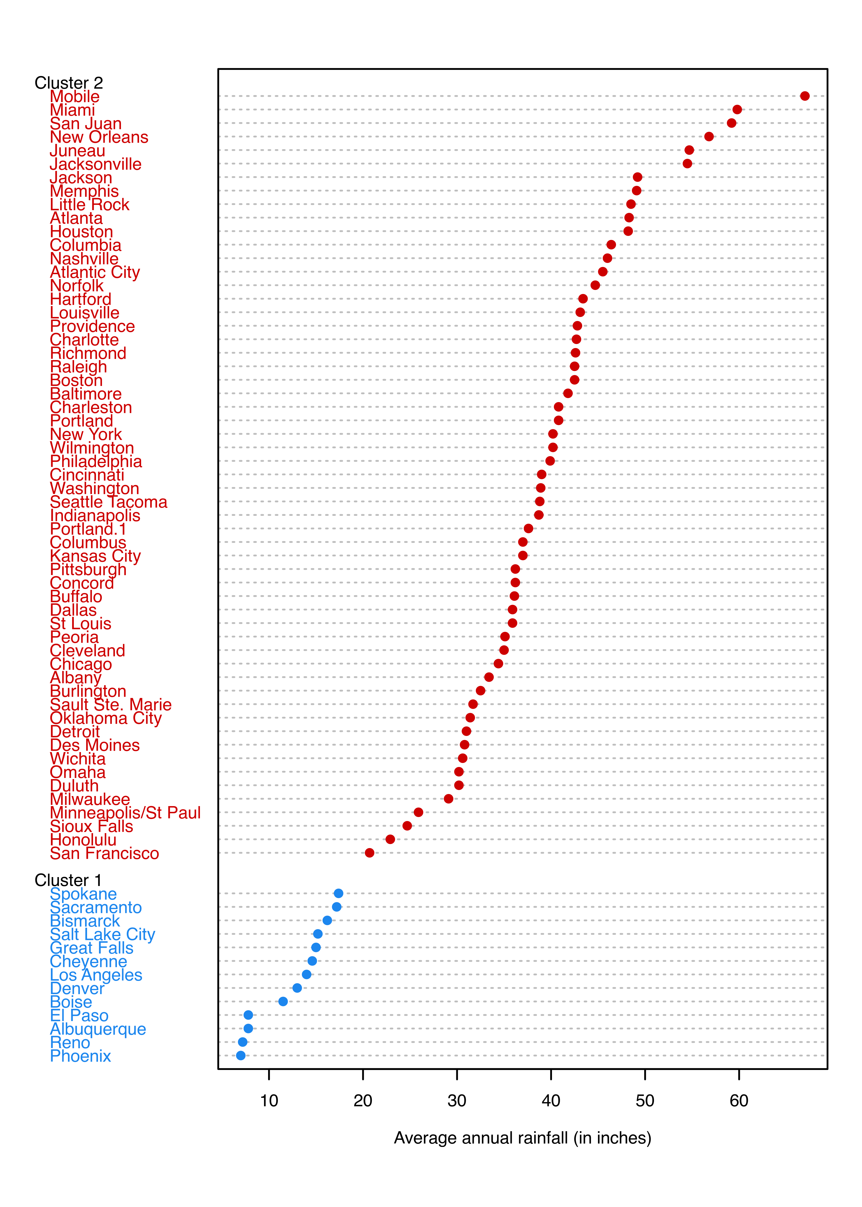
Each of the graphs shown indicates that the two groups of cities are separated by about 20 inches of annual rainfall.
Further graphical capabilities for univariate data are discussed in Section 6.1.
3.6 Model-Based Agglomerative Hierarchical Clustering
Model-based agglomerative hierarchical clustering (MBAHC, Banfield and Raftery 1993) adopts the general ideas of classical agglomerative hierarchical clustering, with the aim of obtaining a hierarchy of clusters of \(n\) objects. Given no preliminary information with regard to grouping, agglomerative hierarchical clustering proceeds from \(n\) clusters each containing a single observation, to one cluster containing all \(n\) observations, by successively merging observations and clusters. In the traditional approach, two groups are merged if they are closest according to a particular distance metric and type of linkage, while in MBAHC, the two groups are merged that optimize a regularized criterion (Fraley 1998) derived from the classification likelihood over all possible merge pairs.
Given \(n\) observations \((\boldsymbol{x}_1, \dots, \boldsymbol{x}_n)\), let \((\ell_1, \dots, \ell_n){}^{\!\top}\) denote the classification labels, so that \(\ell_i=k\) if \(\boldsymbol{x}_i\) is assigned to cluster \(k\). The unknown parameters are obtained by maximizing the classification likelihood: \[ L_{CL}(\boldsymbol{\theta}_1, \dots, \boldsymbol{\theta}_G, \ell_1, \dots, \ell_n ; \boldsymbol{x}_1, \dots, \boldsymbol{x}_n) = \prod_{i=1}^n f_{\ell_i}(\boldsymbol{x}_i ; \boldsymbol{\theta}_{\ell_i}). \] Assuming a multivariate Gaussian distribution for the data, so that \(f_{\ell_i}(\boldsymbol{x}_i ; \boldsymbol{\theta}_{\ell_i}) = \phi(\boldsymbol{x}_i ; \boldsymbol{\mu}_k,\boldsymbol{\Sigma}_k)\) if \(\ell_i=k\), the classification likelihood is \[ L_{CL}(\boldsymbol{\mu}_1, \dots, \boldsymbol{\mu}_G, \boldsymbol{\Sigma}_1, \dots, \boldsymbol{\Sigma}_G, \ell_1, \dots, \ell_n ; \boldsymbol{x}_1, \dots, \boldsymbol{x}_n) = \\ \prod_{k=1}^G \prod_{i \in \mathcal{I}_k} \phi(\boldsymbol{x}_i ; \boldsymbol{\mu}_k,\boldsymbol{\Sigma}_k), \] where \(\mathcal{I}_k = \{ i : \ell_i = k \}\) is the set of indices corresponding to the observations that belong to cluster \(k\). After replacing the unknown mean vectors \(\boldsymbol{\mu}_k\) by their MLEs, \(\widehat{\boldsymbol{\mu}}_k = \bar{\boldsymbol{x}}_k\), the profile (or concentrated) log-likelihood is given by \[ \begin{multline} \log L_{CL}(\boldsymbol{\Sigma}_1, \dots, \boldsymbol{\Sigma}_G, \ell_1, \dots, \ell_n ; \boldsymbol{x}_1, \dots, \boldsymbol{x}_n) = \\ -\frac{1}{2} nd \log(2\pi) -\frac{1}{2} \sum_{k=1}^G \{ \tr(\boldsymbol{W}_k \boldsymbol{\Sigma}_k^{-1}) + n_k \log|\boldsymbol{\Sigma}_k| \}, \end{multline} \tag{3.1}\] where \(\boldsymbol{W}_k = \sum_{i \in \mathcal{I}_k} (\boldsymbol{x}_i - \bar{\boldsymbol{x}}_k)(\boldsymbol{x}_i - \bar{\boldsymbol{x}}_k){}^{\!\top}\) is the sample cross-product matrix for the \(k\)th cluster, and \(n_k\) is the number of observations in cluster \(k\).
By imposing different covariance structures on \(\boldsymbol{\Sigma}_k\), different merging criteria can be derived (see Fraley 1998, Table 1). For instance, assuming a common isotropic cluster-covariance, \(\boldsymbol{\Sigma}_k = \sigma^2\boldsymbol{I}\), the log-likelihood in Equation 3.1 is maximized by minimizing the criterion \[ \tr\left( \sum_{k=1}^G \boldsymbol{W}_k \right), \] the well-known sum of squares criterion of Ward (1963). If the covariances are allowed to be different across clusters, then the criterion to be minimized at each stage of the hierarchical algorithm is \[ \sum_{k=1}^G n_k \log \left| \frac{\boldsymbol{W}_k}{n_k} \right|. \] Methods for regularizing these criteria and efficient numerical algorithms for their minimization have been discussed by Fraley (1998). Table 3.1 lists the models for hierarchical clustering available in mclust.
At each stage of MBAHC, a pair of groups is merged that minimizes a regularized merge criterion over all possible merge pairs (Fraley 1998). Regularization is necessary because cluster contributions to the merge criterion (and the classification likelihood) are undefined for singletons, as well as for other combinations of observations resulting in a singular or near-singular sample covariance.
Traditional hierarchical clustering procedures, as implemented, for example, in the base R function hclust(), are typically represented graphically with a dendrogram that shows the links between objects using a tree diagram, usually with the root at the top and leaves at the bottom. The height of the branches reflects the order in which the clusters are joined, and, to some extent, it also reflects the distances between clusters (see, for example, Hastie, Tibshirani, and Friedman 2009, sec. 14.3.12).
Because the regularized merge criterion may either increase or decrease from stage to stage, the association of a positive distance with merges in traditional hierarchical clustering does not apply to MBAHC. However, it is still possible to draw a dendrogram in the which the tree height increases as the number of groups decreases, so that the root is at the top of the hierarchy. Moreover, the classification likelihood often increases in the later stages of merging (small numbers of clusters), in which case the corresponding dendrogram can be drawn.
mclust provides the function hc() to perform model-based agglomerative hierarchical clustering. It takes the data matrix to be clustered as the main argument. The principal optional arguments are as follows:
modelName: for selecting the model to fit among the four models available, which, following the nomenclature in Table 2.1, are denoted asEII,VII,EEE, andVVV(default).partition: for providing an initial partition from which to start the agglomeration. The default is to start with partitioning into unique observations.use: for specifying the data transformation to apply before performing hierarchical clustering. By defaultuse = "VARS", so the variables are expressed in the original scale. Other possible values, including the default for initialization of the EM algorithm in model-based clustering, are described in Section 3.7.
Example 3.9 Model-based hierarchical cluastering of European unemployment data
Consider the EuroUnemployment dataset which provides unemployment rates for 31 European countries for the year 2014. The considered rates are shown in the table below.
| Variable | Description |
|---|---|
TUR |
Total unemployment rate, defined as the percentage of unemployed persons aged 15–74 in the economically active population. |
YUR |
Youth unemployment rate, defined as the percentage of unemployed persons aged 15–24 in the economically active population. |
LUR |
Long-term unemployment rate, defined as the percentage of unemployed persons who have been unemployed for 12 months or more. |
data("EuroUnemployment", package = "mclust")
summary(EuroUnemployment)
##       TUR             YUR            LUR
##  Min.   : 3.50   Min.   : 7.7   Min.   : 0.60
##  1st Qu.: 6.35   1st Qu.:15.4   1st Qu.: 2.10
##  Median : 8.70   Median :20.5   Median : 3.70
##  Mean   :10.05   Mean   :23.2   Mean   : 4.86
##  3rd Qu.:11.35   3rd Qu.:24.1   3rd Qu.: 6.80
##  Max.   :26.50   Max.   :53.2   Max.   :19.50
The following code fits the isotropic EII and unconstrained VVV agglomerative hierarchical clustering models to this data:
HC_EII = hc(EuroUnemployment, modelName = "EII")
HC_VVV = hc(EuroUnemployment, modelName = "VVV")
Merge dendrograms (with uniform length between the hierarchy levels) for the EII and VVV models are plotted and shown in Figure 3.26.
plot(HC_EII, what = "merge", labels = TRUE, hang = 0.02)
plot(HC_VVV, what = "merge", labels = TRUE, hang = 0.02)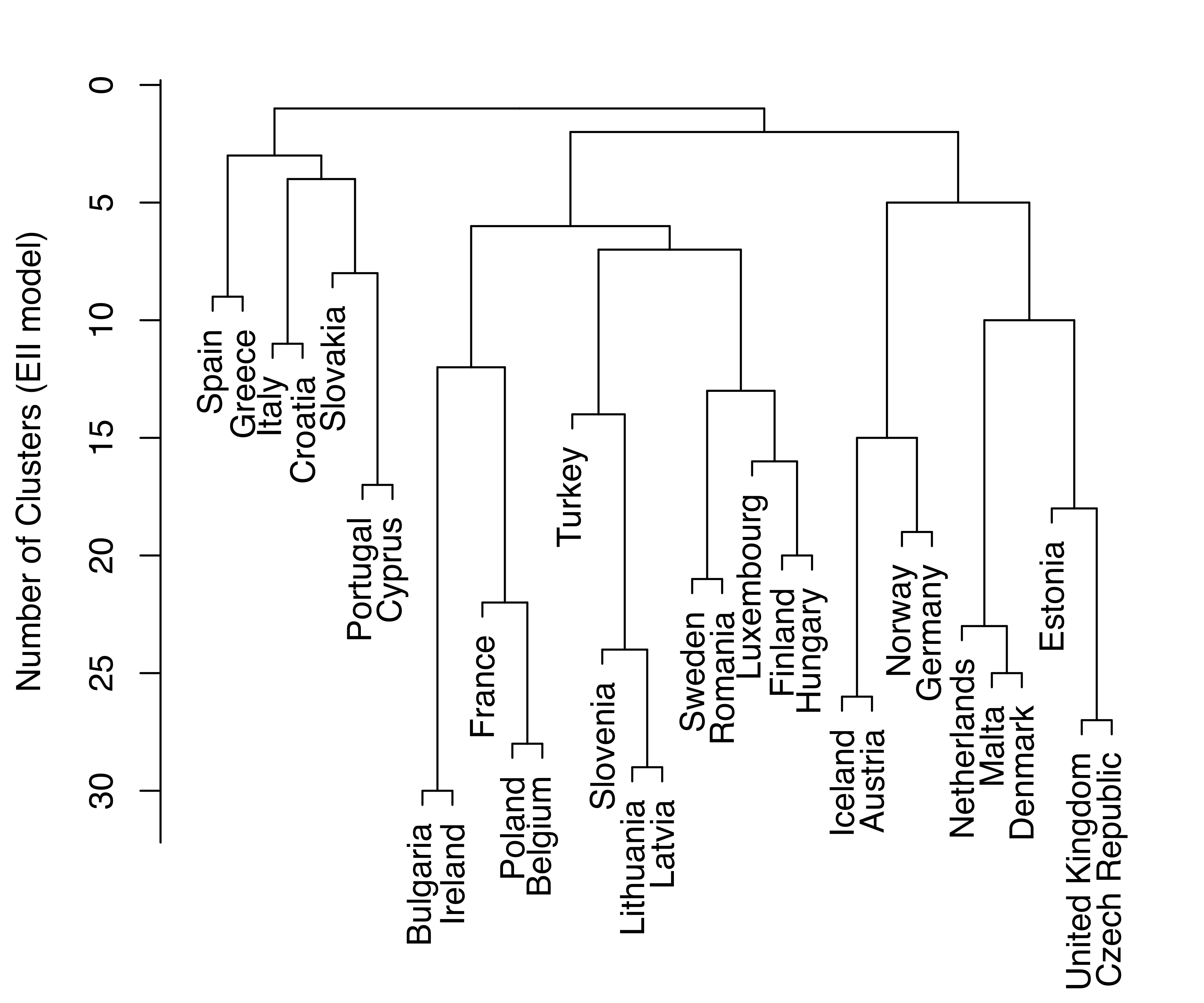
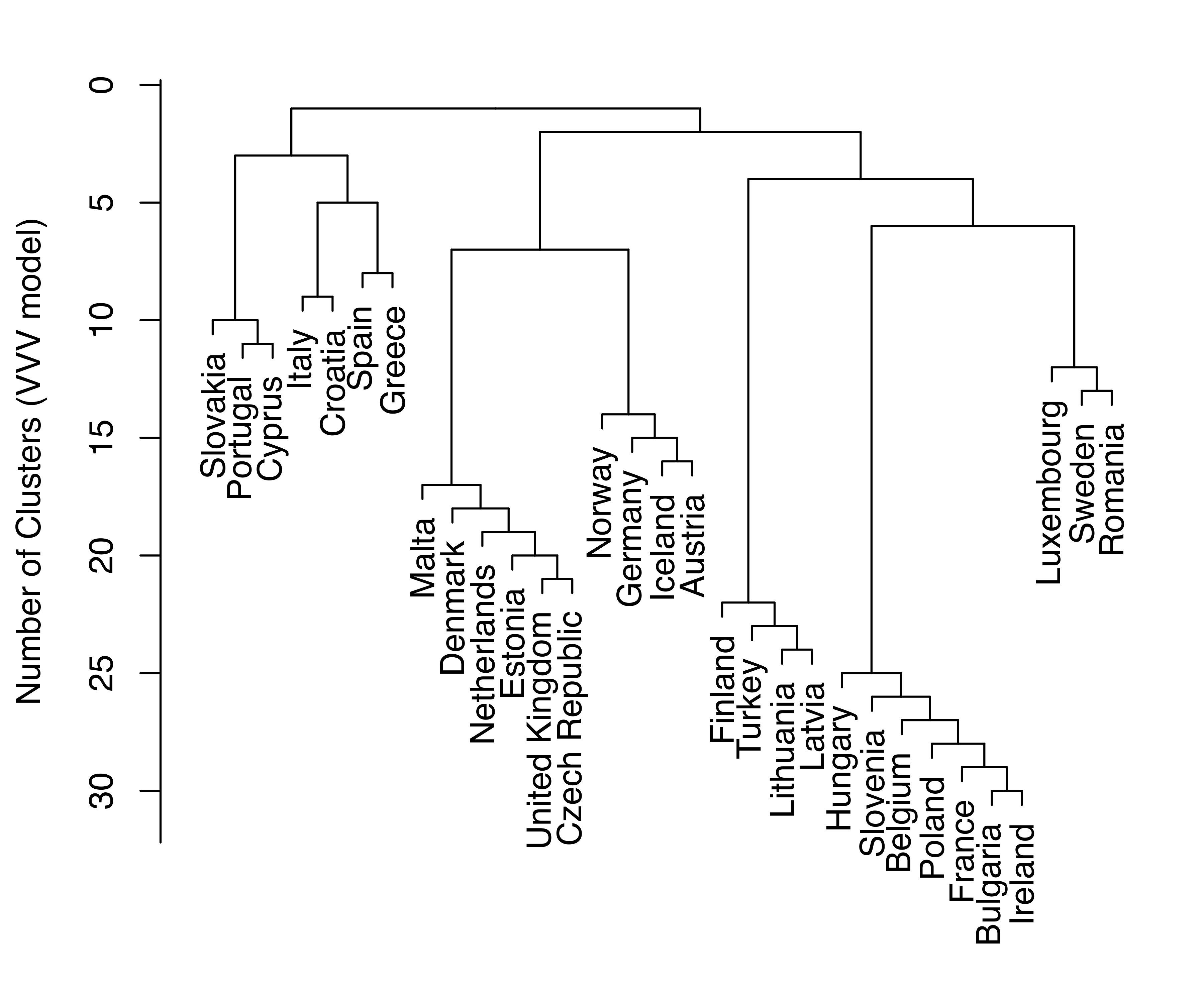
EuroUnemployment data with the EII (a) and VVV (b) models.
Log-likelihood dendrograms for the EII and VVV models are plotted and shown in Figure 3.27. These dendrograms extend from one cluster only as far as the classification likelihood increases and is defined (no singletons or singular covariances).
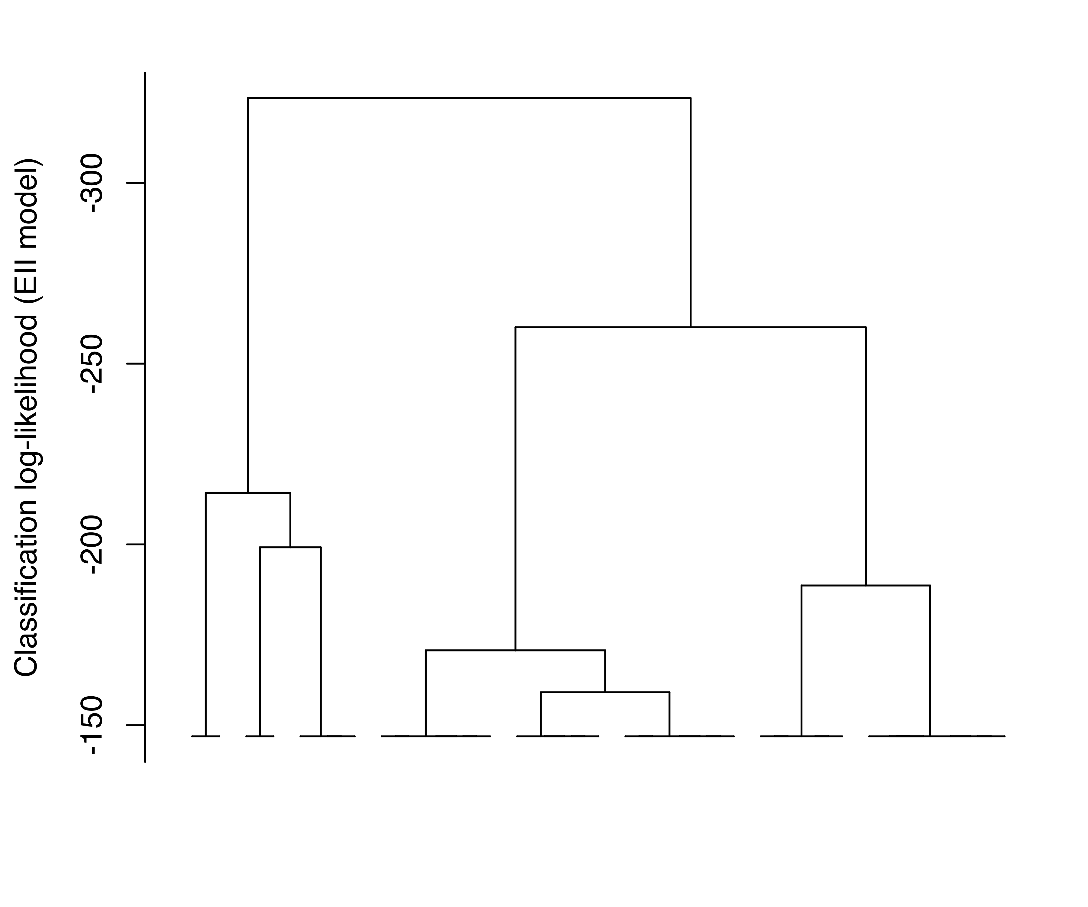
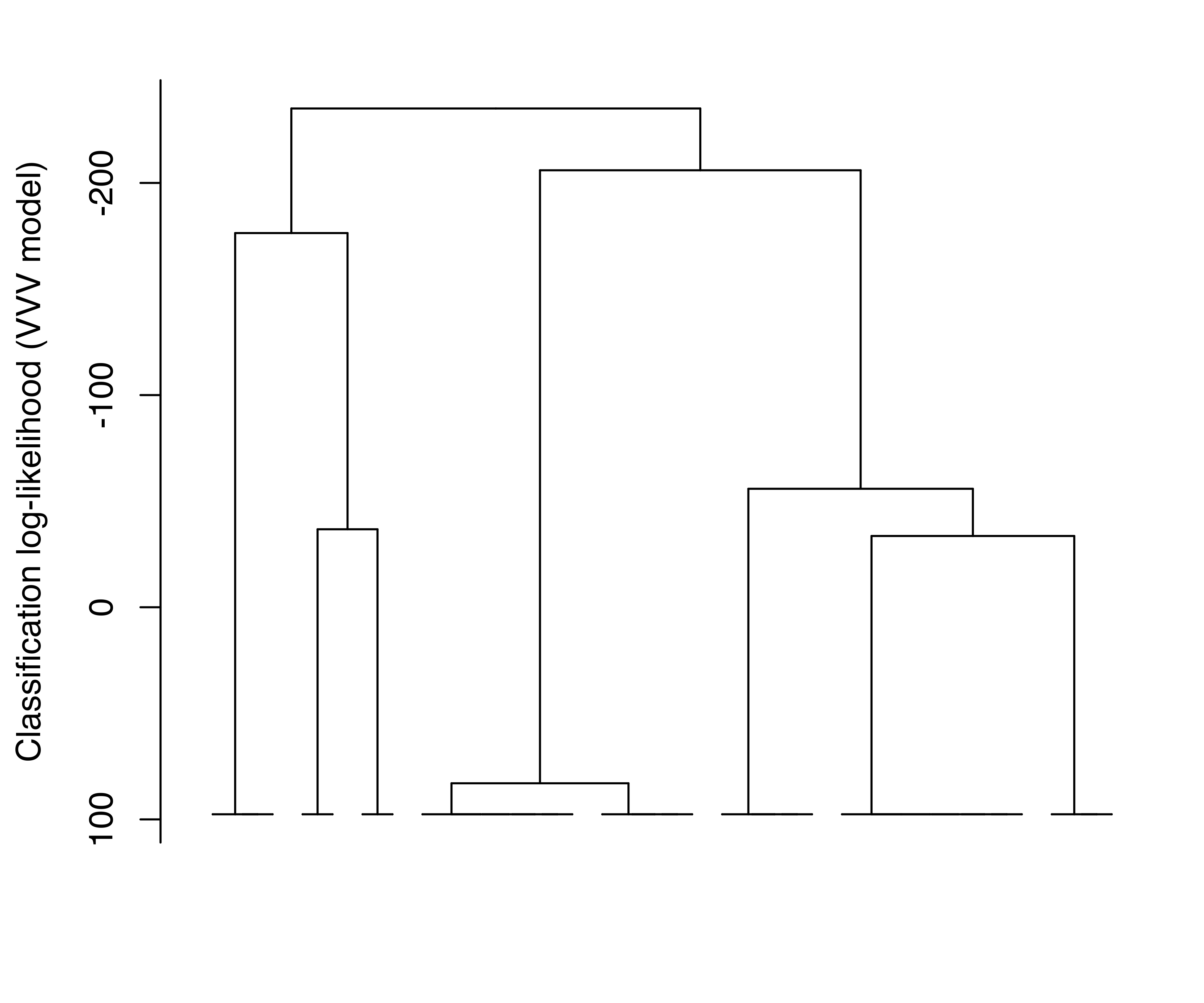
EuroUnemployment data with the EII (a) and VVV (b) models. The log-likelihood is undefined at the other levels of the trees due to the presence of singletons.
3.6.1 Agglomerative Clustering for Large Datasets
Model-based hierarchical agglomerative clustering is computationally demanding on large datasets, both in terms of time and memory. However, it is possible to initialize the modeling from a partition containing fewer groups than the number of observations. For example, Posse (2001) proposed using a subgraph of the minimum spanning tree associated with the data to derive an initial partition for model-based hierarchical clustering. He illustrated the method by applying it to a multiband MRI image of the human brain and to data on global precipitation climatology.
The optional argument partition available in the function hc() allows us to specify an initial partition of observations from which to start the agglomeration process.
Example 3.10 Model-based hierarchical clustering on star data
As a simple illustration, consider the HRstars dataset from the GDAdata package (Unwin 2015), which contains 6,200 measurements of star data on four variables. We first use \(k\)-means to divide the data into 100 groups, and then apply MBAHC to the data with this initial partition.
data("HRstars", package = "GDAdata")
set.seed(0)
initial = kmeans(HRstars[, -1], centers = 100, nstart=10)$cluster
HC_VVV = hc(HRstars[, -1], modelName = "VVV",
            partition = initial, use = "VARS")
HC_VVV
## Call:
## hc(data = HRstars[, -1], modelName = "VVV", use = "VARS", partition =
## initial)
##
## Model-Based Agglomerative Hierarchical Clustering
## Model name        = VVV
## Use               = VARS
## Number of objects = 6220
3.7 Initialization in mclust
As discussed in Section 2.2.3, initialization of the EM algorithm in model-based clustering is often crucial, because the likelihood surfaces for models of interest tend to have many local maxima and may even be unbounded, not to mention having regions where progress is slow. In mclust, the EM algorithm for multivariate data is initialized with the partitions obtained from model-based agglomerative hierarchical clustering (MBAHC), by default using the unconstrained (VVV) model. Efficient numerical algorithms for agglomerative hierarchical clustering with multivariate normal models have been discussed by Fraley (1998) and briefly reviewed in Section 3.6. In this approach, the two clusters are merged that yield the minimum regularized merge criterion (derived from the classification likelihood) over all possible merges at the current stage of the procedure.
Using unconstrained MBAHC is particularly convenient for GMMs because the underlying probability model (VVV) is shared to some extent by both the initialization step and the model fitting step. This strategy also has the advantage in that it provides the basis for initializing EM for any number of mixture components and component-covariance parameterizations. Although there is no guarantee that EM when so initialized will converge to a finite local optimum, it often provides reasonable starting values.
An issue with hierarchical clustering methods is that the resolution of ties in the merge criterion can have a significant effect on the downstream clustering outcome. Such ties are not uncommon when the data are discrete or when continuous data are rounded. Moreover, as the merges progress, these ties may not be exact for numerical reasons, and as a consequence results may be sensitive to relatively small changes in the data, including the order of the variables.
One way of detecting sensitivity in the results of a clustering method is to apply it to perturbed data. Such perturbations can be implemented in a number of ways, such as jittering the data, changing the order of the variables, or comparing results on different subsets of the data when there are a sufficient number of observations. Iterative methods, such as EM, can be initialized with different starting values.
Example 3.11 Clustering flea beatle data
As an illustration of the issues related to the initialization of the EM algorithm, consider the flea beatle data available in package tourr (Wickham and Cook 2022). This dataset provides six physical measurements for a sample of 74 fleas from three species as shown in the table below.
| Variable | Description |
|---|---|
species |
Species of flea beetle from the genus Chaetocnema: concinna, heptapotamica, heikertingeri. |
tars1 |
Width of the first joint of the first tarsus in microns (the sum of measurements for both tarsi) |
tars2 |
Width of the second joint of the first tarsus in microns (the sum of measurements for both tarsi) |
head |
Maximal width of the head between the external edges of the eyes (in \(0.01\) mm). |
ade1 |
Maximal width of the aedeagus in the fore-part (in microns). |
ade2 |
Front angle of the aedeagus (1 unit = \(7.5\) degrees) |
ade3 |
Aedeagus width from the side (in microns). |
data("flea", package = "tourr")
X = data.matrix(flea[, 1:6])
Class = factor(flea$species,
               labels = c("Concinna", "Heikertingeri", "Heptapotamica"))
table(Class)
## Class
##      Concinna Heikertingeri Heptapotamica
##            21            31            22
Figure 3.28, obtained with the code below, shows the scatterplot matrix of variables in the flea dataset with points marked according to the flea species. Since the observed values are rounded (to the nearest integer presumably), there is a considerable overplotting of points. For this reason, we added transparency (or opacity) to cluster colors via the alpha channel in the following plot:
col = mclust.options("classPlotColors")
clp = clPairs(X, Class, lower.panel = NULL, gap = 0,
              symbols = c(16, 15, 17),
              colors = adjustcolor(col, alpha.f = 0.5))
clPairsLegend(x = 0.1, y = 0.3, class = clp$class,
              col = col, pch = clp$pch,
              title = "Flea beatle species")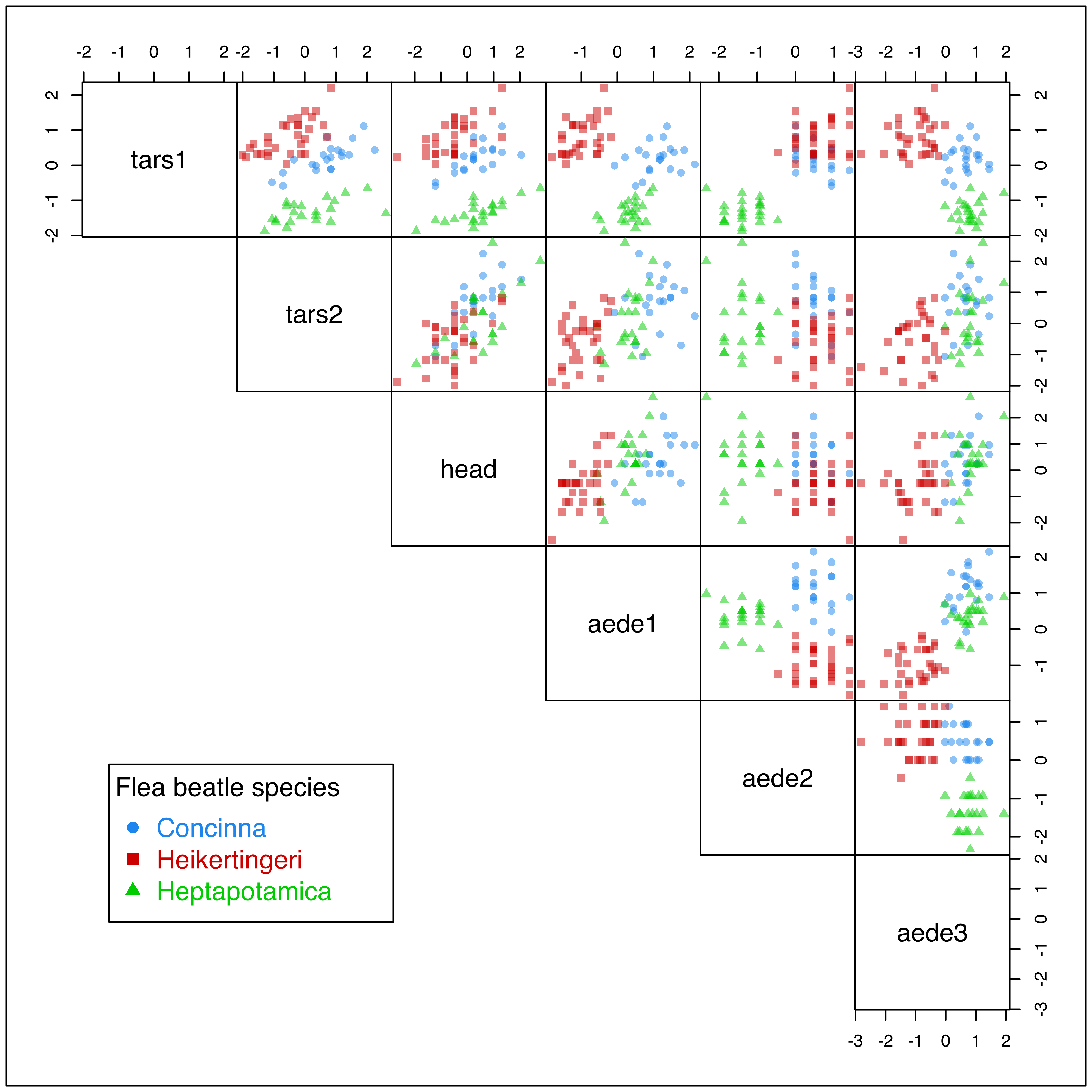
flea dataset with points marked according to the true classes.
Luca Scrucca et al. (2016) discussed model-based clustering for this dataset and showed that using the original variables for the MBAHC initialization step leads to sub-optimal results in Mclust().
# set the default for the current session
mclust.options("hcUse" = "VARS")
mod1 = Mclust(X)
# or specify the initialization method only for this model
# mod1 = Mclust(X, initialization = list(hcPairs = hc(X, use = "VARS")))
summary(mod1)
## ----------------------------------------------------
## Gaussian finite mixture model fitted by EM algorithm
## ----------------------------------------------------
##
## Mclust EEE (ellipsoidal, equal volume, shape and orientation) model
## with 3 components:
##
##  log-likelihood  n df     BIC    ICL
##         -395.01 74 41 -966.49 -966.5
##
## Clustering table:
##  1  2  3
## 21 22 31
table(Class, mod1$classification)
##
## Class            1  2  3
##   Concinna      21  0  0
##   Heikertingeri  0  0 31
##   Heptapotamica  0 22  0
adjustedRandIndex(Class, mod1$classification)
## [1] 1
If we reverse the order of the variables in the fit, MBAHC yields a different set of initial partitions for EM, a consequence of the discrete nature of the data. With this initialization, Mclust still chooses the EEE model with 5 components, but with a different clustering partition.
mod2 = Mclust(X[, 6:1])
summary(mod2)
## ----------------------------------------------------
## Gaussian finite mixture model fitted by EM algorithm
## ----------------------------------------------------
##
## Mclust EEE (ellipsoidal, equal volume, shape and orientation) model
## with 3 components:
##
##  log-likelihood  n df     BIC    ICL
##         -395.01 74 41 -966.49 -966.5
##
## Clustering table:
##  1  2  3
## 21 22 31
table(Class, mod2$classification)
##
## Class            1  2  3
##   Concinna      21  0  0
##   Heikertingeri  0  0 31
##   Heptapotamica  0 22  0
adjustedRandIndex(Class, mod2$classification)
## [1] 1
This second model has a higher BIC and better clustering accuracy.
In order to assess the stability of the results, we randomly start the EM algorithm using the function hcRandomPairs() to obtain a random hierarchical partitioning of the data for initialization:
mod3 = Mclust(X, initialization = list(hcPairs = hcRandomPairs(X, seed = 1)))
summary(mod3)
## ----------------------------------------------------
## Gaussian finite mixture model fitted by EM algorithm
## ----------------------------------------------------
##
## Mclust VEE (ellipsoidal, equal shape and orientation) model with 4
## components:
##
##  log-likelihood  n df     BIC     ICL
##         -385.73 74 51 -990.98 -991.14
##
## Clustering table:
##  1  2  3  4
## 28 22  3 21
table(Class, mod3$classification)
##
## Class            1  2  3  4
##   Concinna       0  0  0 21
##   Heikertingeri 28  0  3  0
##   Heptapotamica  0 22  0  0
adjustedRandIndex(Class, mod3$classification)
## [1] 0.9286
In this case, we obtain the VEE model with 4 components, which has a lower BIC but a higher ARI compared to the previous model. The function mclustBICupdate() can be used to retain the best models for each combination of number of components and cluster-covariance parameterization across several replications:
BIC = NULL
for (i in 1:50)
{
  # get BIC table from initial random start
  BIC0 = mclustBIC(X, verbose = FALSE,
                   initialization = list(hcPairs = hcRandomPairs(X)))
  # update BIC table by merging best BIC values for each
  # G and modelNames
  BIC  = mclustBICupdate(BIC, BIC0)
}
summary(BIC, k = 5)
## Best BIC values:
##            EEE,3     VEE,3    EEE,4    VVE,4   VEE,4
## BIC      -966.49 -970.3464 -977.888 -986.025 -991.67
## BIC diff    0.00   -3.8529  -11.394  -19.531  -25.18
We can then recover the best model object by a subsequent call to Mclust:
mod4 = Mclust(X, x = BIC)
summary(mod4)
## ----------------------------------------------------
## Gaussian finite mixture model fitted by EM algorithm
## ----------------------------------------------------
##
## Mclust EEE (ellipsoidal, equal volume, shape and orientation) model
## with 3 components:
##
##  log-likelihood  n df     BIC    ICL
##         -395.01 74 41 -966.49 -966.5
##
## Clustering table:
##  1  2  3
## 31 22 21
table(Class, mod4$classification)
##
## Class            1  2  3
##   Concinna       0  0 21
##   Heikertingeri 31  0  0
##   Heptapotamica  0 22  0
adjustedRandIndex(Class, mod4$classification)
## [1] 1
The above procedure is able to identify the true clustering structure, but it is a time-consuming process which for large datasets may not be feasible. Moreover, even when using multiple random starts, there is no guarantee that the best solution found is the best that can be achieved.
L. Scrucca and Raftery (2015) discussed several approaches to improve the hierarchical clustering initialization for model-based clustering. The main idea is to apply a transformation to the data in an effort to enhance separation among clusters before applying the MBAHC for the initialization step. The EM algorithm is then run using the data on the original scale. Among the studied transformations, one that often worked reasonably well (and is used as the default in mclust) is the scaled SVD transformation.
Let \(\boldsymbol{X}\) be the \((n \times p)\) data matrix, and \(\mathbb{X}= (\boldsymbol{X}- \boldsymbol{1}_n\bar{\boldsymbol{x}}{}^{\!\top})\boldsymbol{S}^{-1/2}\) be the corresponding centered and scaled matrix, where \(\bar{\boldsymbol{x}}\) is the vector of sample means, \(\boldsymbol{1}_n\) is the unit vector of length \(n\), and \(\boldsymbol{S}= \diag(s^2_1, \dots, s^2_d)\) is the diagonal matrix of sample variances. Consider the following singular value decomposition (SVD): \[ \mathbb{X}= \boldsymbol{U}\boldsymbol{\Omega}\boldsymbol{V}{}^{\!\top}= \sum_{i=1}^r \omega_i\boldsymbol{u}_i\boldsymbol{v}{}^{\!\top}_i, \] where \(\boldsymbol{u}_i\) are the left singular vectors, \(\boldsymbol{v}_i\) the right singular vectors, \(\omega_1 \ge \omega_2 \ge \dots \ge \omega_r > 0\) the corresponding singular values, and \(r \le \min(n,d)\) the rank of matrix \(\mathbb{X}\), with equality when there are no singularities. The scaled SVD transformation is computed as: \[ \boldsymbol{\mathscr{X}}= \mathbb{X}\boldsymbol{S}^{-1/2} \boldsymbol{V}\boldsymbol{\Omega}^{-1/2} = \boldsymbol{U}\boldsymbol{\Omega}^{1/2}, \] for which \(\Exp(\boldsymbol{\mathscr{X}}) = \boldsymbol{0}\) and \(\Var(\boldsymbol{\mathscr{X}}) = \boldsymbol{\Omega}/n = \diag(\omega_i)/n\). Thus, in the transformed scale the features are centered, uncorrelated, and with decreasing variances equal to the square root of the eigenvalues of the marginal sample correlation matrix.
Example 3.12 Clustering flea beatle data (continued)
A GMM estimation initialized using MBAHC with the scaled SVD transformation of the data described above is obtained with the following code:
mclust.options("hcUse" = "SVD")  # restore the default
mod5 = Mclust(X) # X is the unscaled flea data
# or specify only for this model fit
# mod5 = Mclust(X, initialization = list(hcPairs = hc(X, use = "SVD")))
summary(mod5)
## ----------------------------------------------------
## Gaussian finite mixture model fitted by EM algorithm
## ----------------------------------------------------
##
## Mclust EEE (ellipsoidal, equal volume, shape and orientation) model
## with 3 components:
##
##  log-likelihood  n df     BIC    ICL
##         -395.01 74 41 -966.49 -966.5
##
## Clustering table:
##  1  2  3
## 21 31 22
table(Class, mod5$classification)
##
## Class            1  2  3
##   Concinna      21  0  0
##   Heikertingeri  0 31  0
##   Heptapotamica  0  0 22
adjustedRandIndex(Class, mod5$classification)
## [1] 1
In this case, a single run with the scaled SVD initialization strategy (the default strategy for the Mclust() function) yields the highest BIC, and a perfect classification of the fleas into the actual species. However, as the true clustering would not usually be known, analysis with perturbations and/or multiple initialization strategies is always advisable.
With EM, it is possible to do model-based clustering starting with parameter estimates, conditional probabilities, or classifications other than those produced by model-based agglomerative hierarchical clustering. The next section provides some further details on how to run an EM algorithm for Gaussian mixtures in mclust.
3.8 EM Algorithm in mclust
As described in Section 2.2.2, an iteration of EM consists of an E-step and an M-step. The E-step computes a matrix \(\boldsymbol{Z}=\{z_{ik}\}\), where \(z_{ik}\) is an estimate of the conditional probability that observation \(i\) belongs to cluster \(k\) given the current parameter estimates. The M-step computes parameter estimates given \(\boldsymbol{Z}\).
mclust provides functions em() and me() implementing the EM algorithm for maximum likelihood estimation in Gaussian mixture models for all 14 of the covariance parameterizations based on eigen-decomposition. The em() function starts with the E-step; besides the data and model specification, the model parameters (means, covariances, and mixing proportions) must be provided. The me() function, on the other hand, starts with the M-step; besides the data and model specification, the matrix of conditional probabilities must be provided. The output for both are the maximum likelihood estimates of the model parameters and the matrix of conditional probabilities.
Functions estep() and mstep() implement the individual E- and M- steps, respectively, of an EM iteration. Conditional probabilities and the log-likelihood can be recovered from parameters via estep(), while parameters can be recovered from conditional probabilities using mstep().
Example 3.13 Single M- and E- steps using the iris data
Consider the well-known iris dataset (Anderson 1935, Fisher:1936) which contains the measurements (in cm) of sepal length and width, and petal length and width, for 50 flowers from each of 3 species of Iris, namely setosa, versicolor, and virginica.
The following code shows how single M- and E- steps can be performed using functions mstep() and estep():
data("iris", package = "datasets")
str(iris)
## 'data.frame':    150 obs. of  5 variables:
## $ Sepal.Length: num 5.1 4.9 4.7 4.6 5 5.4 4.6 5 4.4 4.9 ...
## $ Sepal.Width : num 3.5 3 3.2 3.1 3.6 3.9 3.4 3.4 2.9 3.1 ...
## $ Petal.Length: num 1.4 1.4 1.3 1.5 1.4 1.7 1.4 1.5 1.4 1.5 ...
## $ Petal.Width : num 0.2 0.2 0.2 0.2 0.2 0.4 0.3 0.2 0.2 0.1 ...
## $ Species : Factor w/ 3 levels "setosa","versicolor",..: 1 1 1 1 1 1 1
##    1 1 1 ...
ms = mstep(iris[, 1:4], modelName = "VVV",
            z = unmap(iris$Species))
str(ms, 1)
## List of 7
## $ modelName : chr "VVV"
## $ prior : NULL
## $ n : int 150
## $ d : int 4
## $ G : int 3
## $ z : num [1:150, 1:3] 1 1 1 1 1 1 1 1 1 1 ...
## ..- attr(*, "dimnames")=List of 2
## $ parameters:List of 3
## - attr(*, "returnCode")= num 0
es = estep(iris[, 1:4], modelName = "VVV",
            parameters = ms$parameters)
str(es, 1)
## List of 7
## $ modelName : chr "VVV"
## $ n : int 150
## $ d : int 4
## $ G : int 3
## $ z : num [1:150, 1:3] 1 1 1 1 1 1 1 1 1 1 ...
## ..- attr(*, "dimnames")=List of 2
## $ parameters:List of 3
## $ loglik : num -183
## - attr(*, "returnCode")= num 0
In this example, the initial estimate of z for the M-step is a matrix of indicator variables corresponding to a discrete classification taken from the true classes contained in iris$Species. Here, we used the function unmap() to convert the classification into the corresponding matrix of indicator variables. The inverse function, called map(), converts a matrix in which each row sums to 1 into an integer vector specifying for each row the column index of the maximum. This last operation is basically the MAP when applied to the matrix of posterior conditional probabilities (see Section 2.2.4).
3.9 Further Considerations in Cluster Analysis via Mixture Modeling
Clustering can be affected by control parameter settings, such as convergence tolerances within the clustering functions, although the defaults are often adequate.
Control parameters used by the EM functions in mclust are set and retrieved using the function emControl(), These include:
eps: A tolerance value for terminating iterations due to ill-conditioning, such as near singularity in covariance matrices. By default this is set to.Machine$double.eps, the relative machine precision, which has the value2.220446e-16on IEEE-compliant machines.tol: A vector of length 2 giving iteration convergence tolerances. By default this is set toc(1.0e-5, sqrt(.Machine$double.eps)). The first value is the tolerance for the relative convergence of the log-likelihood in the EM algorithm, and the second value is the relative convergence tolerance for the M-step of those models that have an iterative M-step, namely the modelsVEI,EVE,VEE,VVE, andVEV(see Table 2.2).itmax: An integer vector of length two giving integer limits on the number of EM iterations and on the number of iterations in the inner loop for models with iterative M-step (see above). By default this is set toc(.Machine$integer.max, .Machine$integer.max), allowing termination to be completely governed by the control parametertol. A warning is issued if this limit is reached before the convergence criterion is satisfied.
Although these control settings are in a sense hidden by the defaults, they may have a significant effect on results in some instances and should be taken into consideration in any analysis.
The mclust implementation includes various warning messages in cases of potential problems. These are issued if mclust.options("warn") is set to TRUE or specified directly in function calls. Note, however, that by default mclust.options("warn") = FALSE, so that these warning messages are suppressed.
Finally, it is important to take into account numerical issues in model-based cluster analysis, and more generally in GMM estimation. The computations for estimating the model parameters break down when the covariance corresponding to one or more components becomes ill-conditioned (singular or nearly singular), and cannot proceed if clusters contain only a few observations or if the observations they contain are nearly colinear. Estimation may also fail when one or more mixing proportions shrink to negligible values. Including a prior is often helpful in such situations (see Section 7.2).