7 Miscellanea
\[ \DeclareMathOperator{\Real}{\mathbb{R}} \DeclareMathOperator{\Proj}{\text{P}} \DeclareMathOperator{\Exp}{\text{E}} \DeclareMathOperator{\Var}{\text{Var}} \DeclareMathOperator{\var}{\text{var}} \DeclareMathOperator{\sd}{\text{sd}} \DeclareMathOperator{\cov}{\text{cov}} \DeclareMathOperator{\cor}{\text{cor}} \DeclareMathOperator{\range}{\text{range}} \DeclareMathOperator{\rank}{\text{rank}} \DeclareMathOperator{\ind}{\perp\hspace*{-1.1ex}\perp} \DeclareMathOperator{\CE}{\text{CE}} \DeclareMathOperator{\BS}{\text{BS}} \DeclareMathOperator{\ECM}{\text{ECM}} \DeclareMathOperator{\BSS}{\text{BSS}} \DeclareMathOperator{\WSS}{\text{WSS}} \DeclareMathOperator{\TSS}{\text{TSS}} \DeclareMathOperator{\BIC}{\text{BIC}} \DeclareMathOperator{\ICL}{\text{ICL}} \DeclareMathOperator{\CV}{\text{CV}} \DeclareMathOperator{\diag}{\text{diag}} \DeclareMathOperator{\se}{\text{se}} \DeclareMathOperator{\Cov}{\text{Cov}} \DeclareMathOperator{\boot}{\text{boot}} \DeclareMathOperator{\LRTS}{\text{LRTS}} \DeclareMathOperator{\Model}{\mathcal{M}} \DeclareMathOperator*{\argmin}{arg\min} \DeclareMathOperator*{\argmax}{arg\max} \DeclareMathOperator{\vech}{vech} \DeclareMathOperator{\tr}{tr} \]
In this chapter a range of other issues is discussed, including accounting for outliers and noise. The use of Bayesian methods is presented for avoiding singularities in mixture modeling by adding a prior. The problem of non-Gaussian clusters is addressed by introducing two approaches, one based on combining Gaussian mixture components according to an entropy criterion and one based on identifying connected components. Simulation from mixture models is also discussed briefly, as well as handling of large datasets, high-dimensional data, and missing data. Several data examples are used for illustrating the implementation of the methods in mclust.
7.1 Accounting for Noise and Outliers
In the finite mixture framework, noisy data are characterized by the presence of outlying observations that do not belong to any mixture component. There are two main ways to accommodate noise and outliers in a mixture model:
Adding one or more components to the mixture to represent noise and modifying the EM algorithm accordingly to estimate parameters (Dasgupta and Raftery 1998; C. Fraley and Raftery 1998).
Modeling by mixtures of distributions with heavier tails than the Gaussian, such as a mixture of \(t\) distributions (McLachlan and Peel 2000).
Some other alternatives for robust Gaussian mixture modeling are proposed in Garcı́a-Escudero et al. (2008), Punzo and McNicholas (2016), Coretto and Hennig (2016), and Dotto and Farcomeni (2019).
In mclust, the strategy for accommodating noise is to include a constant–rate Poisson process mixture component to represent the noise, resulting in the following mixture log-likelihood \[ \ell(\boldsymbol{\Psi}, \pi_0) = \sum_{i=1}^n \log \left\{ \frac{\pi_0}{V} + \sum_{k=1}^{G} \pi_k \phi (\boldsymbol{x}_i \mid \boldsymbol{\mu}_k, \boldsymbol{\Sigma}_k) \right\}, \tag{7.1}\] where \(V\) is the hypervolume of the data region, and \(\pi_k \ge 0\) are the mixing weights under the constraint \(\sum_{k=0}^{G} \pi_k = 1\). An observation contributes \(1/V\) to the likelihood if it belongs to the noise component; otherwise its contribution comes from the Gaussian components. This model has been used successfully in a number of applications (Banfield and Raftery 1993; Dasgupta and Raftery 1998; J. Campbell et al. 1997; J. G. Campbell et al. 1999).
The model-fitting procedure is as follows. Given a preliminary noise assignment for the observations, model-based hierarchical clustering is applied to the correspondingly denoised data to obtain initial clustering partitions for the Gaussian portion of the mixture model. EM is then initialized, using the preliminary noise, together with the hierarchical clustering assignment for each number of clusters specified.
The effectiveness of this approach hinges on obtaining a good initial specification of the noise. Some possible strategies for initial denoising include methods based on Voronoï tessellation (Allard and Fraley 1997), nearest neighbors (Byers and Raftery 1998), and robust covariance estimation (Wang and Raftery 2002).
Example 7.1 Clustering with noisy minefields data
Dasgupta and Raftery (1998) discussed the problem of detecting surface-laid minefields from an aircraft image. The main goal was to distinguish the mines from the clutter (metal objects or rocks). As an example, consider the simulated minefield data with clutter analyzed in C. Fraley and Raftery (1998) and available in mclust.
data("chevron", package = "mclust")
summary(chevron)
##    class           x                y
##  data :350   Min.   :  1.18   Min.   :  1.01
##  noise:754   1st Qu.: 34.39   1st Qu.: 27.51
##              Median : 58.82   Median : 49.50
##              Mean   : 61.09   Mean   : 56.71
##              3rd Qu.: 86.52   3rd Qu.: 86.67
##              Max.   :127.49   Max.   :127.86
noise = with(chevron, class == "noise")
X = chevron[,2:3]
plot(X, cex = 0.5)
plot(X, cex = 0.5, col = ifelse(noise, "grey", "black"),
pch = ifelse(noise, 3, 1))The plot of simulated minefield data is shown in panel (a) of Figure 7.1, while panel (b) displays the dataset with noise (clutter) marked by a grey cross. Note that about 70% of the data points are clutter, and the true minefield is contained within the chevron-shaped area, consisting of two intersecting rectangles.
To include noise in modeling with Mclust() or mclustBIC(), an initial guess of the noise observations must be supplied via the noise component of the initialization argument. The function NNclean() in the R package prabclus (Hennig and Hausdorf 2020) is an implementation of the methodology proposed by Byers and Raftery (1998). Under the assumption that the noise is distributed as a homogeneous Poisson point process and that the remaining data is also distributed as a homogeneous Poisson process but with higher intensity on a (possibly disconnected) subregion, the observed \(k\)th nearest neighbor distances are modeled as a mixture of two transformed Gamma distributions with parameters estimated by the EM algorithm. The observed points can then be assigned to either the noise or higher-density component depending on the estimated posterior probabilities.
This example uses \(k=5\) nearest neighbors to detect the noise, which amounts to \(662/1104 \approx 60\%\) of the observed data points. The resulting denoised data is shown in Figure 7.2 (a)}. With this initial estimate of the noise, a GMM is fitted with the following code:
The model-based clustering procedure with the noise component selects the (EEV,2) model, closely followed by the (EVE,2) model. In both cases two clusters are correctly identified. A summary of the estimated model with the highest BIC and the corresponding classification plot are obtained as follows:
summary(modNoise, parameters = TRUE)
## ----------------------------------------------------
## Gaussian finite mixture model fitted by EM algorithm
## ----------------------------------------------------
##
## Mclust EEV (ellipsoidal, equal volume and shape) model with 2
## components and a noise term:
##
##  log-likelihood    n df    BIC    ICL
##          -10525 1104 11 -21128 -21507
##
## Clustering table:
##   1   2   0
## 160 151 793
##
## Mixing probabilities:
##       1       2       0
## 0.12290 0.12618 0.75091
##
## Means:
##     [,1]   [,2]
## x 71.473 39.519
## y 36.310 31.566
##
## Variances:
## [,,1]
##         x       y
## x  195.85 -176.99
## y -176.99  197.30
## [,,2]
##        x      y
## x 183.00 176.47
## y 176.47 210.15
##
## Hypervolume of noise component:
## 16022
addmargins(table(chevron$class, modNoise$classification), 2)
##
##           0   1   2 Sum
##   data   50 156 144 350
##   noise 743   4   7 754
plot(modNoise, what = "classification")
The summary output consists of the usual statistics for the selected GMM, plus an estimate of the hypervolume associated with the noise component. The classification obtained is shown in Figure 7.2, which reflects the generating process for the data quite well. The cross-tabulation of the estimated classification and the known data labels shows that most of the clutter is correctly identified, as is the true minefield. The sensitivity is \(= 743/754 = 98.54\%\), and the specificity is \(= (156+144)/350 = 85.71\%\).
By default mclust uses the function hypvol() to compute the hypervolume \(V\) in Equation 7.1. This gives a simple approximation to the hypervolume of a multivariate dataset by taking the minimum of the volume hyperrectangle (box) containing the observed data and the box obtained from principal components. In other words, the estimate is the minimum of the Cartesian product of the variable intervals and the Cartesian product of the corresponding projection onto principal components.
hypvol(X)
## [1] 16022
Another option is to compute the ellipsoid hull, namely the ellipsoid of minimal volume such that all observed points lie either inside or on the boundary of the ellipsoid. This method is available via the function ellipsoidhull() from the cluster R package (Maechler et al. 2022):
library("cluster")
ehull = ellipsoidhull(as.matrix(X))
volume(ehull)
## [1] 23150
modNoise.ehull = Mclust(X, Vinv = 1/volume(ehull),
                         initialization = list(noise = (nnc$z == 0)))
summary(modNoise.ehull)
## ----------------------------------------------------
## Gaussian finite mixture model fitted by EM algorithm
## ----------------------------------------------------
##
## Mclust VVE (ellipsoidal, equal orientation) model with 3 components and
## a noise term:
##
##  log-likelihood    n df    BIC    ICL
##          -10777 1104 17 -21673 -22618
##
## Clustering table:
##   1   2   3   0
## 187 192 302 423
tab = table(chevron$class, modNoise.ehull$classification)
addmargins(tab, 2)
##
##           0   1   2   3 Sum
##   data    0 164 164  22 350
##   noise 423  23  28 280 754
In this case the number of clusters identified is too large, yielding a poor recovery of the noise component (sensitivity \(= 423/754 = 56.1\%\), and specificity \(= (164+164+22)/350 = 100\%\)). This behavior is a consequence of the ellipsoid hull over-estimating the data volume (to be expected because the noise is distributed over a square, so that a larger volume ellipsoid is needed to contain all the data points). The hyperrectangle approach discussed above would in all cases be a better approximation to the data volume than the ellipsoid hull. However, the volume of the convex hull of the data better approximates the data volume than either of these approaches.
The following code obtains the volume of the convex hull for the bivariate minefield simulated data, using the convhulln() function from package geometry (Habel et al. 2022):
library("geometry")
chull = convhulln(X, options = "FA")
chull$vol
## [1] 15828
The reciprocal of this value may be used as input for the argument Vinv of function Mclust():
modNoise.chull = Mclust(X, Vinv = 1/chull$vol,
                        initialization = list(noise = (nnc$z == 0)))
summary(modNoise.chull)
## ----------------------------------------------------
## Gaussian finite mixture model fitted by EM algorithm
## ----------------------------------------------------
##
## Mclust EEV (ellipsoidal, equal volume and shape) model with 2
## components and a noise term:
##
##  log-likelihood    n df    BIC    ICL
##          -10515 1104 11 -21108 -21487
##
## Clustering table:
##   1   2   0
## 157 149 798
tab = table(chevron$class, modNoise.chull$classification)
addmargins(tab, 2)
##
##           0   1   2 Sum
##   data   55 153 142 350
##   noise 743   4   7 754
For this dataset, the default value of the hypervolume and that computed using convhulln() are quite close, so the corresponding estimated models provide essentially the same fit.
An issue with the convex hull is that it may not be practical to compute in high dimensions. Moreover, implementations without the option to return the logarithm could result in overflow or underflow depending on the scaling of the data.
Other strategies for obtaining an initial noise estimate could be adopted. The function cov.nnve() in the contributed R package covRobust (Wang, Raftery, and Fraley 2017) is an implementation of robust covariance estimation via nearest neighbor cleaning (Wang and Raftery 2002). An example of its usage is the following:
For the case of \(k = 5\) nearest neighbors, only \(5/1104 \approx 0.05\%\) of data is classified as noise. A relatively good clustering model is nevertheless obtained with this initial estimate of the noise:
modNoise.nnve = Mclust(X, initialization =
                       list(noise = (nnve$classification == 0)))
summary(modNoise.nnve$BIC)
## Best BIC values:
##           EEV,2        EVE,2       EVV,2
## BIC      -21128 -21128.20252 -21134.8273
## BIC diff      0     -0.36423     -6.9891
summary(modNoise.nnve)
## ----------------------------------------------------
## Gaussian finite mixture model fitted by EM algorithm
## ----------------------------------------------------
##
## Mclust EEV (ellipsoidal, equal volume and shape) model with 2
## components and a noise term:
##
##  log-likelihood    n df    BIC    ICL
##          -10525 1104 11 -21128 -21509
##
## Clustering table:
##   1   2   0
## 160 150 794
addmargins(table(chevron$class, modNoise.nnve$classification), 2)
##
##           0   1   2 Sum
##   data   51 153 146 350
##   noise 743   7   4 754
Although the final model is somewhat different from the one previously selected, this one also has 2 components, and the classification of data as signal or noise is almost identical (sensitivity \(= 743/754 = 98.54\%\), and specificity \(= (153+146)/350 = 85.43\%\)). By increasing the number of nearest neighbors \(k\) for the initial noise estimate, the results for the cov.nnve() denoising approach those obtained with NNclean.
Example 7.2 Clustering with outliers on simulated data
Peel and McLachlan (2000) developed a simulation-based example in the context of fitting of mixtures of (multivariate) \(t\) distributions to model data containing observations with longer than normal tails or atypical observations. The data used in their example is generated as follows:
(Sigma = array(c(2, 0.5, 0.5, 0.5, 1, 0, 0, 0.1, 2, -0.5, -0.5, 0.5),
                dim = c(2, 2, 3)))
## , , 1
##
##      [,1] [,2]
## [1,]  2.0  0.5
## [2,]  0.5  0.5
##
## , , 2
##
##      [,1] [,2]
## [1,]    1  0.0
## [2,]    0  0.1
##
## , , 3
##
##      [,1] [,2]
## [1,]  2.0 -0.5
## [2,] -0.5  0.5
var.decomp = sigma2decomp(Sigma)
str(var.decomp)
## List of 7
## $ sigma : num [1:2, 1:2, 1:3] 2 0.5 0.5 0.5 1 0 0 0.1 2 -0.5 ...
## $ d : int 2
## $ modelName : chr "VVI"
## $ G : int 3
## $ scale : num [1:3] 0.866 0.316 0.866
## $ shape : num [1:2, 1:3] 2.484 0.403 3.162 0.316 2.484 ...
## $ orientation: num [1:2, 1:2] -0.957 -0.29 0.29 -0.957
par = list(pro = c(1/3, 1/3, 1/3),
            mean = cbind(c(0, 3), c(3, 0), c(-3, 0)),
            variance = var.decomp)
data = sim(par$variance$modelName, parameters = par, n = 200)
noise = matrix(runif(100, -10, 10), nrow = 50, ncol = 2)
X = rbind(data[, 2:3], noise)
cluster = c(data[, 1], rep(0, 50))
clPairs(X, ifelse(cluster == 0, 0, 1),
        colors = "black", symbols = c(16, 1), cex = c(0.5, 1))
In the code above we used the function sim() to simulate 200 observations from a GMM with the specified mixing probabilities pro, component means mean, and variance decomposition var.decomp obtained using the function sigma2decomp() (see Section 7.4). Then, we added 50 outlying observations from a uniform distribution on \((-10,10)\). The simulated data is shown in Figure 7.3 (a).
We apply the same procedure adopted for noisy data in Example 7.1. We get an initial estimate of the outlying observations with NNclean(), and then we apply Mclust() to all the data using this estimate of noise in the initialization step:
nnc = NNclean(X, k = 5)
modNoise = Mclust(X, initialization = list(noise = (nnc$z == 0)))
summary(modNoise$BIC)
## Best BIC values:
##            VEI,3      VEE,3      VVI,3
## BIC      -2243.8 -2249.2536 -2253.0499
## BIC diff     0.0    -5.4888    -9.2851
summary(modNoise, parameters = TRUE)
## ----------------------------------------------------
## Gaussian finite mixture model fitted by EM algorithm
## ----------------------------------------------------
##
## Mclust VEI (diagonal, equal shape) model with 3 components and a noise
## term:
##
##  log-likelihood   n df     BIC     ICL
##         -1083.2 250 14 -2243.8 -2267.4
##
## Clustering table:
##  1  2  3  0
## 66 63 74 47
##
## Mixing probabilities:
##       1       2       3       0
## 0.25532 0.24244 0.28647 0.21578
##
## Means:
##        [,1]     [,2]     [,3]
## x1 2.968281 -0.40142 -3.13151
## x2 0.022729  3.01644  0.13098
##
## Variances:
## [,,1]
##        x1      x2
## x1 0.7887 0.00000
## x2 0.0000 0.12971
## [,,2]
##       x1      x2
## x1 1.896 0.00000
## x2 0.000 0.31181
## [,,3]
##        x1      x2
## x1 1.9577 0.00000
## x2 0.0000 0.32195
##
## Hypervolume of noise component:
## 377.35
The clusters identified are shown in Figure 7.3 (b), and the following code can be used to plot the result and obtain the confusion matrix:
This shows that the three groups (labeled “1”, “2”, “3”) and the outlying observations (labeled “0”) have been well identified.
7.2 Using a Prior for Regularization
Maximum likelihood estimation for Gaussian mixtures using the EM algorithm may fail as the result of singularities or degeneracies. These problems can arise depending on the data and the starting values for the EM algorithm, as well as the model parameterizations and number of components specified for the mixture.
To address these situations, Chris Fraley and Raftery (2007) proposed replacing the maximum likelihood estimate (MLE) by a maximum a posteriori (MAP) estimate, also estimated by the EM algorithm. A highly dispersed proper conjugate prior is used, containing a small fraction of one observation’s worth of information. The resulting method avoids degeneracies and singularities, but when these are not present it gives similar results to the standard maximum likelihood method. The prior also has the effect of smoothing noisy behavior of the BIC, which is often observed in conjunction with instability in estimation.
For univariate data, a Gaussian prior on the mean (conditional on the variance) is used: \[ \begin{align} \mu \mid \sigma^2 & \sim \mathcal{N}(\mu_{\scriptscriptstyle \mathcal{P}}, \sigma^2/\kappa_{\scriptscriptstyle \mathcal{P}}) \nonumber\\ & \propto \left(\sigma^2\right)^{-\frac{1}{2}} \exp\left\{ - \frac{\kappa_{\scriptscriptstyle \mathcal{P}}}{2\sigma^2} \left(\mu - \mu_{\scriptscriptstyle \mathcal{P}}\right)^2 \right\}, \end{align} \tag{7.2}\] and an inverse gamma prior on the variance: \[ \begin{align} \sigma^2 & \sim \mbox{inverseGamma}(\nu_{\scriptscriptstyle \mathcal{P}}/2, \varsigma^2_{\scriptscriptstyle \mathcal{P}}/2) \nonumber\\ & \propto \left(\sigma^2\right)^{-\frac{\nu_{\scriptscriptstyle \mathcal{P}}+2}{2}} \exp \left\{ -\frac{\varsigma^2_{\scriptscriptstyle \mathcal{P}}}{2\sigma^2} \right\}. \end{align} \tag{7.3}\]
For multivariate data, a Gaussian prior on the mean (conditional on the covariance matrix) is used: \[ \begin{align} \boldsymbol{\mu}\mid \boldsymbol{\Sigma} & \sim \mathcal{N}(\boldsymbol{\mu}_{\scriptscriptstyle \mathcal{P}}, \boldsymbol{\Sigma}/\kappa_{\scriptscriptstyle \mathcal{P}}) \nonumber\\ & \propto \left|\boldsymbol{\Sigma}\right|^{-\frac{1}{2}} \exp\left\{ -\frac{\kappa_{\scriptscriptstyle \mathcal{P}}}{2} \tr\left(\left(\boldsymbol{\mu}- \boldsymbol{\mu}_{\scriptscriptstyle \mathcal{P}}\right){}^{\!\top} \boldsymbol{\Sigma}^{-1} \left(\boldsymbol{\mu}- \boldsymbol{\mu}_{\scriptscriptstyle \mathcal{P}}\right) \right) \right\}, \end{align} \tag{7.4}\] together with an inverse Wishart prior on the covariance matrix: \[ \begin{align} \boldsymbol{\Sigma} & \sim \mbox{inverseWishart}(\nu_{\scriptscriptstyle \mathcal{P}}, \boldsymbol{\Lambda}_{\scriptscriptstyle \mathcal{P}}) \nonumber\\ & \propto \left|\boldsymbol{\Sigma}\right|^{-\frac{\nu_{\scriptscriptstyle \mathcal{P}}+d+1}{2}} \exp\left\{ -\frac{1}{2} \tr\left(\boldsymbol{\Sigma}^{-1} \boldsymbol{\Lambda}_{\scriptscriptstyle \mathcal{P}}^{-1} \right) \right\}. \end{align} \tag{7.5}\]
The hyperparameters \(\mu_{\scriptscriptstyle \mathcal{P}}\) (in the univariate case) or \(\boldsymbol{\mu}_{\scriptscriptstyle \mathcal{P}}\) (in the multivariate case), \(\kappa_{\scriptscriptstyle \mathcal{P}}\), and \(\nu_{\scriptscriptstyle \mathcal{P}}\) are called the mean, shrinkage, and degrees of freedom, respectively. Parameters \(\varsigma^2_{\scriptscriptstyle \mathcal{P}}\) (a scalar, in the univariate case) and \(\boldsymbol{\Lambda}_{\scriptscriptstyle \mathcal{P}}\) (a matrix, in the multivariate case) are the scale of the prior distribution. These priors are called conjugate priors for the normal distribution because the posterior can be expressed as the product of a normal distribution and an inverse gamma or Wishart distribution.
When a prior is included, a modified version of the BIC must be used to select the number of mixture components and the model parameterization. The BIC is computed as described in Section 2.3.1, but with the log-likelihood evaluated at the MAP instead of at the MLE. Further details on model-based clustering using prior distributions can be found in Chris Fraley and Raftery (2007).
7.2.1 Adding a Prior in mclust
Although maximum likelihood estimation is the default, functions such as Mclust() and mclustBIC() have a prior argument that allows specification of a conjugate prior on the means and variances of the type described above. mclust provides two functions to facilitate inclusion of a prior:
priorControl()supplies input for thepriorargument. It gives the name of the function that defines the desired conjugate prior and specifies values for its arguments.defaultPrior()is the default function named inpriorControl(), as well as a template for specifying conjugate priors in mclust.
The defaultPrior() function has the following arguments:
dataA numeric vector, matrix, or data frame of observations.GAn integer value specifying the number of mixture components.modelNameA character string indicating the model to be fitted. Note that in the multivariate case only 10 out of 14 models are available, as indicated in Table 3.1.
The following optional arguments can also be specified:
meanA single value \(\mu_{\scriptscriptstyle \mathcal{P}}\) or a vector \(\boldsymbol{\mu}_{\scriptscriptstyle \mathcal{P}}\) of values for the mean parameter of the prior. By default, the sample mean of each variable is used.shrinkageThe shrinkage parameter \(\kappa_{\scriptscriptstyle \mathcal{P}}\) for the prior on the mean. By default,shrinkage = 0.01. The posterior mean \[ \frac{n_k \bar{\boldsymbol{x}}_k + \kappa_{\scriptscriptstyle \mathcal{P}}\boldsymbol{\mu}_{\scriptscriptstyle \mathcal{P}}}{\kappa_{\scriptscriptstyle \mathcal{P}}+ n_k}, \] can be viewed as adding \(\kappa_{\scriptscriptstyle \mathcal{P}}\) observations with value \(\boldsymbol{\mu}_{\scriptscriptstyle \mathcal{P}}\) to each group in the data. The default value was determined by experimentation; values close to and larger than 1 caused large perturbations in the modeling in cases where there were no missing BIC values without the prior. The value \(\kappa_{\scriptscriptstyle \mathcal{P}}= 0.01\) resulted in BIC curves that appeared to be smooth extensions of their counterparts without the prior. By settingshrinkage = 0orshrinkage = NAno prior is assumed for the mean.dofThe degrees of freedom \(\nu_{\scriptscriptstyle \mathcal{P}}\) for the prior on the variance. By analogy to the univariate case, the marginal prior distribution of \(\boldsymbol{\mu}\) is a \(t\) distribution centered at \(\boldsymbol{\mu}_{\scriptscriptstyle \mathcal{P}}\) with \(\nu_{\scriptscriptstyle \mathcal{P}}- d + 1\) degrees of freedom. The mean of this distribution is \(\boldsymbol{\mu}_{\scriptscriptstyle \mathcal{P}}\) provided that \(\nu_{\scriptscriptstyle \mathcal{P}}> d\), and it has a finite covariance matrix provided \(\nu_{\scriptscriptstyle \mathcal{P}}> d + 1\) (see, for example, Joseph L. Schafer 1997). By default, \(\nu_{\scriptscriptstyle \mathcal{P}}= d+2\), the smallest integer value for the degrees of freedom that gives a finite covariance matrix.scaleThe scale parameter for the prior on the variance.
For univariate models and multivariate spherical or diagonal models, it is computed by default as \[ \varsigma^2_{\scriptscriptstyle \mathcal{P}}= \frac{\tr(\boldsymbol{S})/d}{G^{2/d}}, \] which is the average of the diagonal elements of the empirical covariance matrix \(\boldsymbol{S}\) of the data, divided by the square of the number of components to the \(1/d\) power. This is roughly equivalent to partitioning the range of the data into \(G\) intervals of fairly equal size.
For multivariate ellipsoidal models, it is computed by default as \[ \boldsymbol{\Lambda}_{\scriptscriptstyle \mathcal{P}}= \frac{\boldsymbol{S}}{G^{2/d}}, \] the covariance matrix, divided by the square of the number of components to the \(1/d\) power.
Example 7.3 Density estimation with a prior on the Galaxies data
Consider the data on the estimated velocity (km/sec) of 82 galaxies in the Corona Borealis region from Kathryn Roeder (1990), available in the MASS package (Venables and Ripley 2013; Ripley 2022). The interest lies in the identification of multimodality as evidence for clustering structures in the pattern of expansion.
data("galaxies", package = "MASS")
# now fix a typographical error in the data
# see help("galaxies", package = "MASS")
galaxies[78] = 26960
galaxies = galaxies / 1000
We start the analysis with no prior, but using multiple random starts and retaining the best estimated fit in terms of BIC:
BIC = NULL
for(i in 1:50)
{
BIC0 = mclustBIC(galaxies, verbose = FALSE,
initialization = list(hcPairs = hcRandomPairs(galaxies)))
BIC = mclustBICupdate(BIC, BIC0)
}
summary(BIC, k = 5)
## Best BIC values:
## V,6 V,3 V,5 V,4 E,6
## BIC -440.06 -442.2177 -442.5948 -443.8970 -447.4629
## BIC diff 0.00 -2.1543 -2.5314 -3.8335 -7.3994
plot(BIC)
mod = densityMclust(galaxies, x = BIC)
summary(mod, parameters = TRUE)
## -------------------------------------------------------
## Density estimation via Gaussian finite mixture modeling
## -------------------------------------------------------
##
## Mclust V (univariate, unequal variance) model with 6 components:
##
## log-likelihood n df BIC ICL
## -182.57 82 17 -440.06 -447.6
##
## Mixing probabilities:
## 1 2 3 4 5 6
## 0.403204 0.085366 0.024390 0.024355 0.036585 0.426099
##
## Means:
## 1 2 3 4 5 6
## 19.7881 9.7101 16.1270 26.9775 33.0443 22.9162
##
## Variances:
## 1 2 3 4 5 6
## 0.45348851 0.17851527 0.00184900 0.00030625 0.84956356 1.45114183
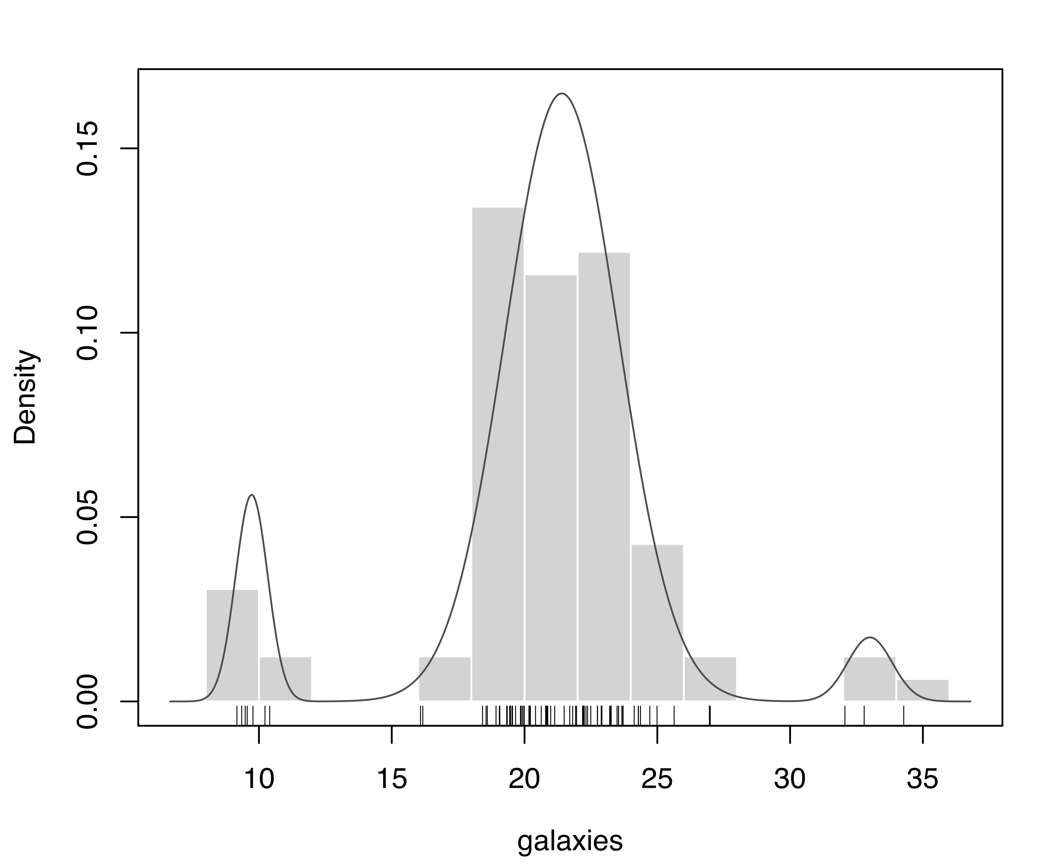
plot(mod, what = "density", data = galaxies, breaks = 11)
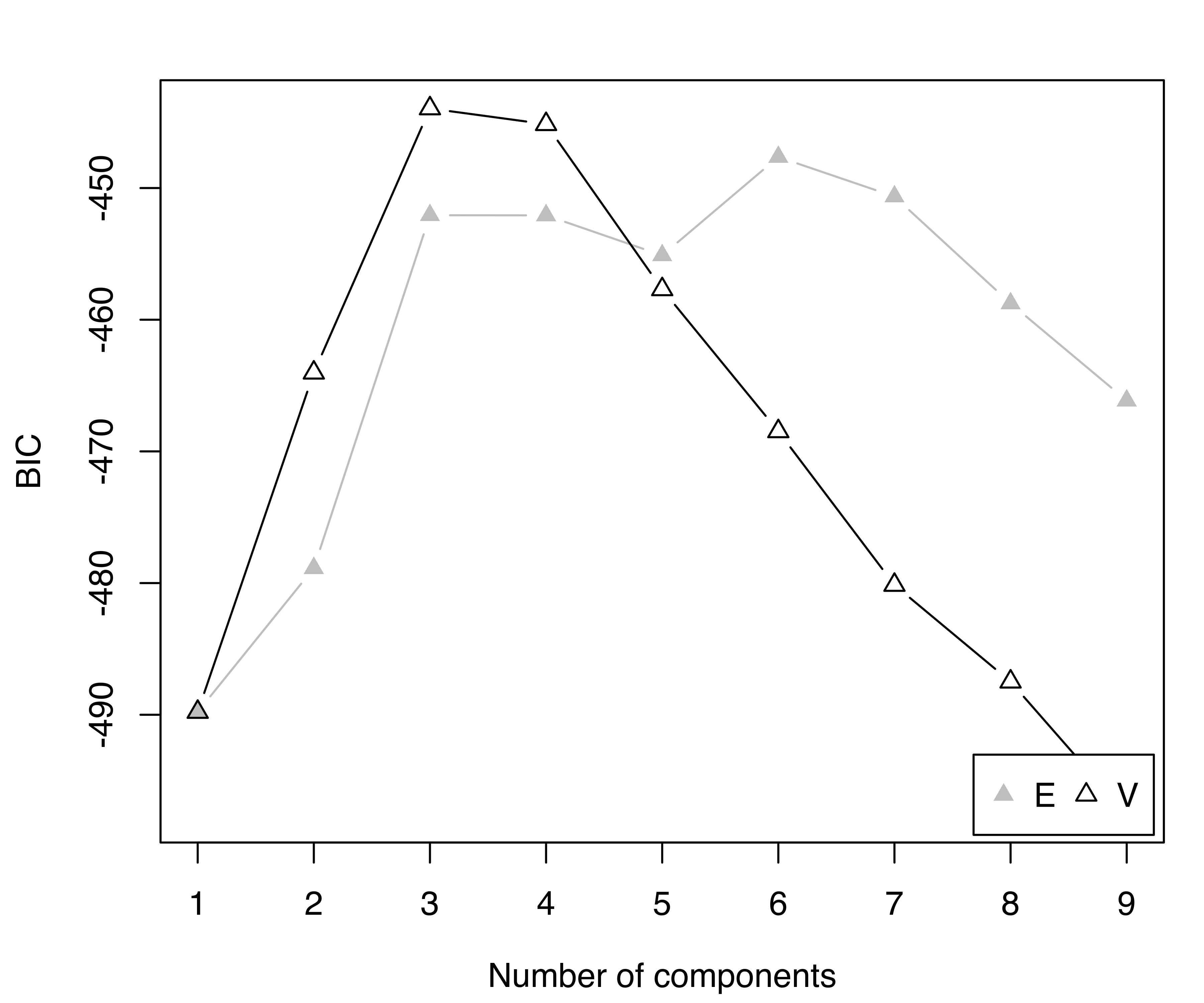
rug(galaxies)The model with the largest BIC has 6 components, each with a different variance. Components with very small mixing weights correspond to narrow spikes in the density estimate (see Figure 7.4), suggesting them to be spurious.
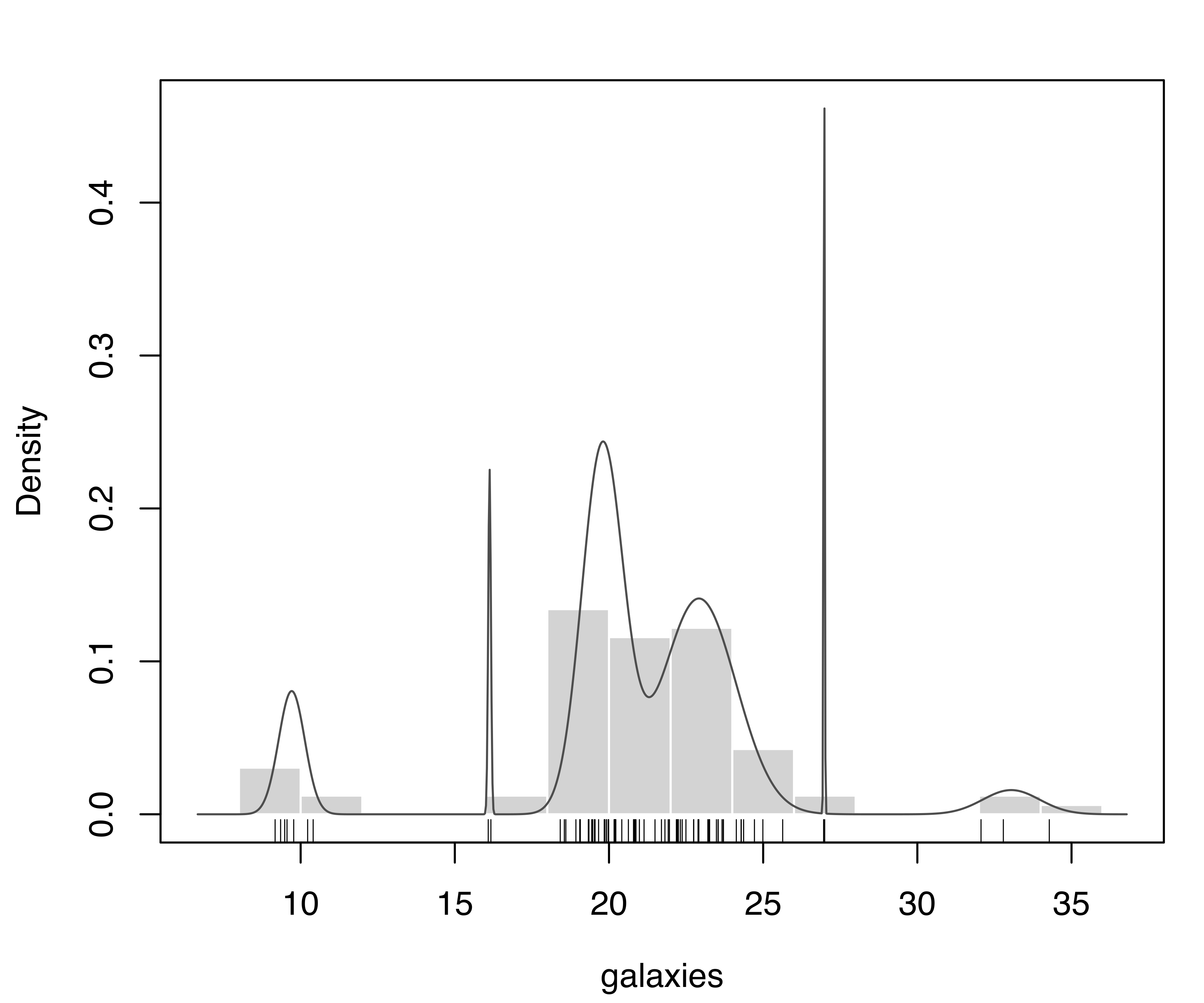
V,6) model selected according to BIC for the galaxies dataset.
The previous analysis can be modified by including the prior as follows:
BICp = NULL
for(i in 1:50)
{
  BIC0p = mclustBIC(galaxies, verbose = FALSE,
                     prior = priorControl(),
            initialization = list(hcPairs = hcRandomPairs(galaxies)))
  BICp  = mclustBICupdate(BICp, BIC0p)
}
summary(BICp, k = 5)
## Best BIC values:
##              V,3      V,4       E,6       E,7       E,3
## BIC      -443.96 -445.153 -447.6407 -450.6451 -452.0662
## BIC diff    0.00   -1.196   -3.6833   -6.6878   -8.1088
plot(BICp)

modp = densityMclust(galaxies, x = BICp)
summary(modp, parameters = TRUE)
## -------------------------------------------------------
## Density estimation via Gaussian finite mixture modeling
## -------------------------------------------------------
##
## Mclust V (univariate, unequal variance) model with 3 components:
##
## Prior: defaultPrior()
##
##  log-likelihood  n df     BIC     ICL
##         -204.35 82  8 -443.96 -443.96
##
## Mixing probabilities:
##        1        2        3
## 0.085366 0.036585 0.878050
##
## Means:
##      1      2      3
##  9.726 33.004 21.404
##
## Variances:
##       1       2       3
## 0.36949 0.70599 4.51272

plot(modp, what = "density", data = galaxies, breaks = 11)
rug(galaxies)
Figure 7.5 shows the BIC trace and the density estimate for the selected model. By including the prior, BIC fairly clearly chooses the model with three components and unequal variances. This is in agreement with other analyses reported in the literature (K. Roeder and Wasserman 1997; Chris Fraley and Raftery 2007).
V,3) model selected according to the BIC (based on the MAP, not the MLE) for the galaxies dataset.
As explained in Section 7.2.1, the function priorControl() is provided for specifying a prior and its parameters. When used with its default settings, it specifies another function called defaultPrior() which can serve as a template for alternative priors. An example of the result of a call to defaultPrior() for the final model selected is shown below:
defaultPrior(galaxies, G = 3, modelName = "V")
## $shrinkage
## [1] 0.01
##
## $mean
## [1] 20.831
##
## $dof
## [1] 3
##
## $scale
## [1] 2.3187
Example 7.4 Clustering with a prior on the Italian olive oils data
Consider the olive oils dataset presented in Example 4.8.
data("olive", package = "pgmm")
# recode of labels for Region and Area
Regions = c("South", "Sardinia", "North")
Areas = c("North Apulia", "Calabria", "South Apulia", "Sicily",
           "Inland Sardinia", "Coastal Sardinia", "East Liguria",
           "West Liguria", "Umbria")
olive$Region = factor(olive$Region, levels = 1:3, labels = Regions)
olive$Area = factor(olive$Area, levels = 1:9, labels = Areas)
with(olive, table(Area, Region))
##                   Region
## Area               South Sardinia North
##   North Apulia        25        0     0
##   Calabria            56        0     0
##   South Apulia       206        0     0
##   Sicily              36        0     0
##   Inland Sardinia      0       65     0
##   Coastal Sardinia     0       33     0
##   East Liguria         0        0    50
##   West Liguria         0        0    50
##   Umbria               0        0    51
We model the data on the standardized scale as follows:
X = scale(olive[, 3:10])
BIC = mclustBIC(X, G = 1:15)
summary(BIC)
## Best BIC values:
## VVE,14 VVE,11 VVE,13
## BIC -4461.6 -4471.3336 -4480.081
## BIC diff 0.0 -9.6941 -18.442
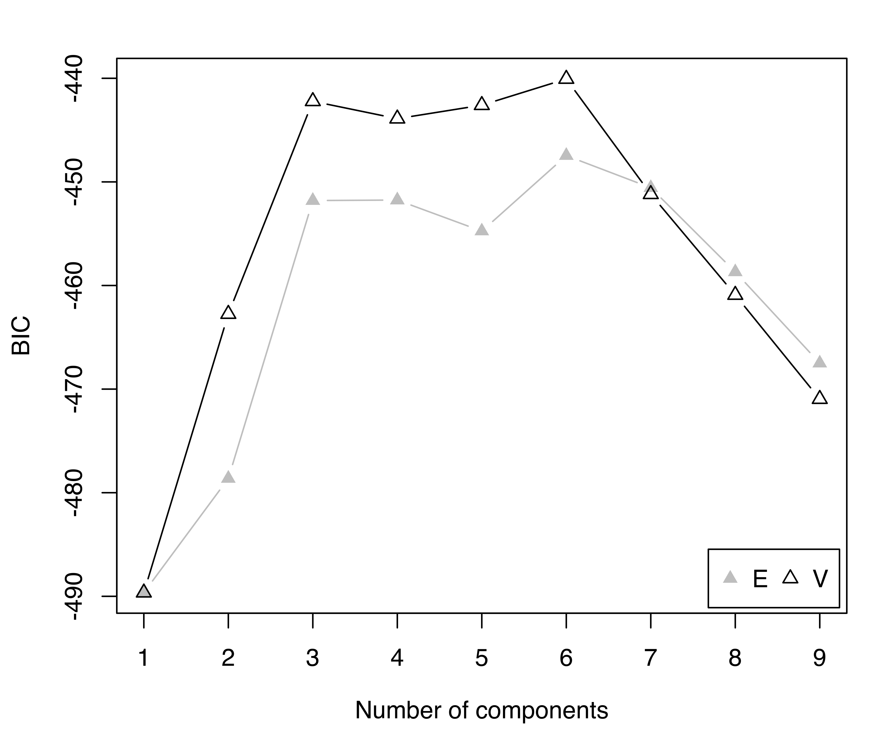
plot(BIC, legendArgs = list(x = "bottomright", ncol = 5))
BICp = mclustBIC(X, G = 1:15, prior = priorControl())
summary(BICp)
## Best BIC values:
## VVV,6 VVV,7 VVV,5
## BIC -5446.7 -5584.27 -5590.59
## BIC diff 0.0 -137.55 -143.86
plot(BICp, legendArgs = list(x = "bottomright", ncol = 5))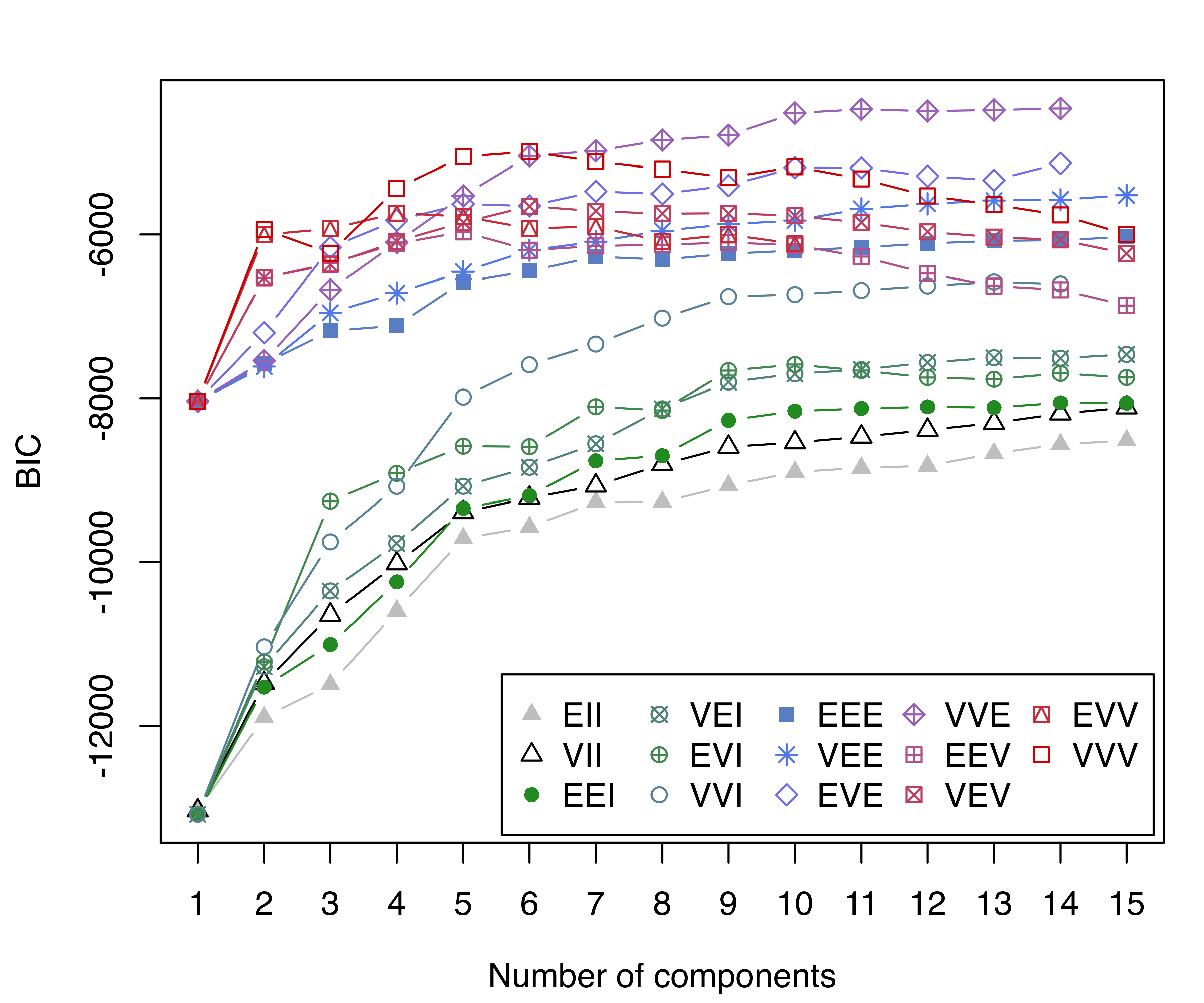
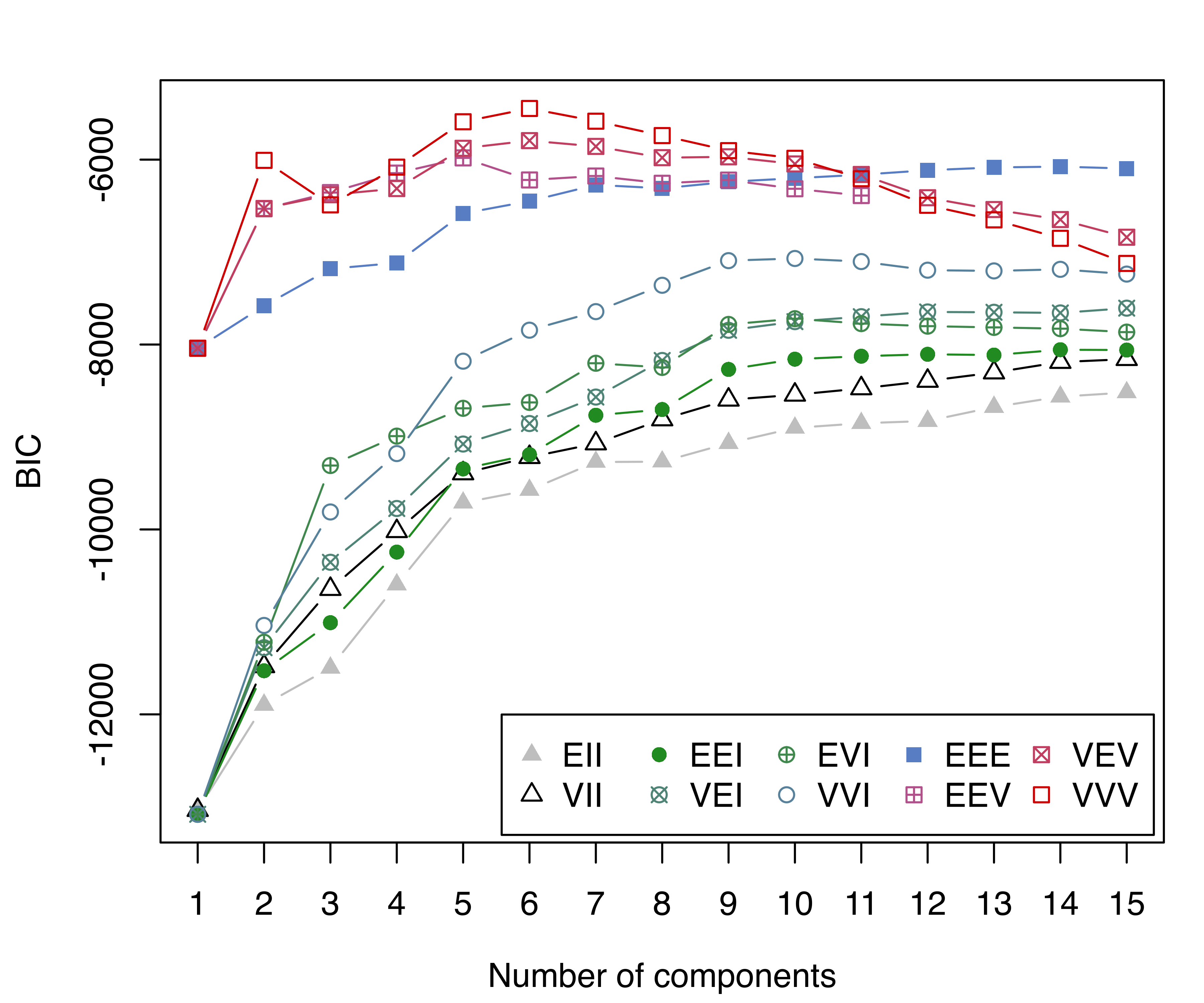
The BIC plots without and with a prior are shown in Figure 7.6. Without a prior, the model selected has a large number of mixture components, and a fairly poor clustering accuracy:
mod = Mclust(X, x = BIC)
summary(mod)
## ----------------------------------------------------
## Gaussian finite mixture model fitted by EM algorithm
## ----------------------------------------------------
##
## Mclust VVE (ellipsoidal, equal orientation) model with 14 components:
##
##  log-likelihood   n  df     BIC     ICL
##         -1389.6 572 265 -4461.6 -4504.4
##
## Clustering table:
##  1  2  3  4  5  6  7  8  9 10 11 12 13 14
## 29 51 34 65 54 90 66 32 11 29 16 41 38 16

table(Region = olive$Region, cluster = mod$classification)
##           cluster
## Region      1  2  3  4  5  6  7  8  9 10 11 12 13 14
##   South    29 51 34 65 54 90  0  0  0  0  0  0  0  0
##   Sardinia  0  0  0  0  0  0 66 32  0  0  0  0  0  0
##   North     0  0  0  0  0  0  0  0 11 29 16 41 38 16
adjustedRandIndex(olive$Region, mod$classification)
## [1] 0.24185

table(Area = olive$Area, cluster = mod$classification)
##                   cluster
## Area                1  2  3  4  5  6  7  8  9 10 11 12 13 14
##   North Apulia     23  0  1  1  0  0  0  0  0  0  0  0  0  0
##   Calabria          0 48  2  6  0  0  0  0  0  0  0  0  0  0
##   South Apulia      0  0  6 57 53 90  0  0  0  0  0  0  0  0
##   Sicily            6  3 25  1  1  0  0  0  0  0  0  0  0  0
##   Inland Sardinia   0  0  0  0  0  0 65  0  0  0  0  0  0  0
##   Coastal Sardinia  0  0  0  0  0  0  1 32  0  0  0  0  0  0
##   East Liguria      0  0  0  0  0  0  0  0  0  1  4 41  4  0
##   West Liguria      0  0  0  0  0  0  0  0  0  0  0  0 34 16
##   Umbria            0  0  0  0  0  0  0  0 11 28 12  0  0  0
adjustedRandIndex(olive$Area, mod$classification)
## [1] 0.54197
The model selected when the prior is included has 6 components with unconstrained variances and a much improved clustering accuracy:
modp = Mclust(X, x = BICp)
summary(modp)
## ----------------------------------------------------
## Gaussian finite mixture model fitted by EM algorithm
## ----------------------------------------------------
##
## Mclust VVV (ellipsoidal, varying volume, shape, and orientation) model
## with 6 components:
##
## Prior: defaultPrior()
##
##  log-likelihood   n  df     BIC     ICL
##         -1869.4 572 269 -5446.7 -5451.4
##
## Clustering table:
##   1   2   3   4   5   6
## 127 196  98  36  58  57

table(Region = olive$Region, cluster = modp$classification)
##           cluster
## Region       1   2   3   4   5   6
##   South    127 196   0   0   0   0
##   Sardinia   0   0  98   0   0   0
##   North      0   0   0  36  58  57
adjustedRandIndex(olive$Region, modp$classification)
## [1] 0.56313

table(Area = olive$Area, cluster = modp$classification)
##                   cluster
## Area                 1   2   3   4   5   6
##   North Apulia      25   0   0   0   0   0
##   Calabria          56   0   0   0   0   0
##   South Apulia      10 196   0   0   0   0
##   Sicily            36   0   0   0   0   0
##   Inland Sardinia    0   0  65   0   0   0
##   Coastal Sardinia   0   0  33   0   0   0
##   East Liguria       0   0   0   0  43   7
##   West Liguria       0   0   0   0   0  50
##   Umbria             0   0   0  36  15   0
adjustedRandIndex(olive$Area, modp$classification)
## [1] 0.78261
The clusters identified correspond approximately to the areas of origin of the olive oil samples. One cluster encompasses both the inland and coastal areas of Sardinia, and two clusters include the southern regions, with one almost completely composed of the south of Apulia. Another three clusters correspond to northern regions: one for all the olive oils from west Liguria and a few from east Liguria, one mostly composed of east Liguria and a few from Umbria, and the last cluster composed only of olive oils from Umbria.
7.3 Non-Gaussian Clusters from GMMs
Cluster analysis aims to identify groups of similar observations that are relatively separated from each other. In the model-based approach to clustering, data is modeled by a finite mixture of density functions belonging to a given parametric class. Each component is typically associated with a group or cluster. This framework can be extended to non-Gaussian clusters by modeling them with more than one mixture component. This problem was addressed by Baudry et al. (2010), who proposed a method based on an entropy criterion for hierarchically combining mixture components to form clusters. Hennig (2010) also discussed hierarchical merging methods based on unimodality and misclassification probabilities. Another approach based on the identification of cluster cores corresponding to regions of high density is introduced by Scrucca (2016).
7.3.1 Combining Gaussian Mixture Components for Clustering
The function clustCombi() provides a means for obtaining models with clusters represented by multiple mixture components, as illustrated below.
Example 7.5 Merging Gaussian mixture components on simulated data
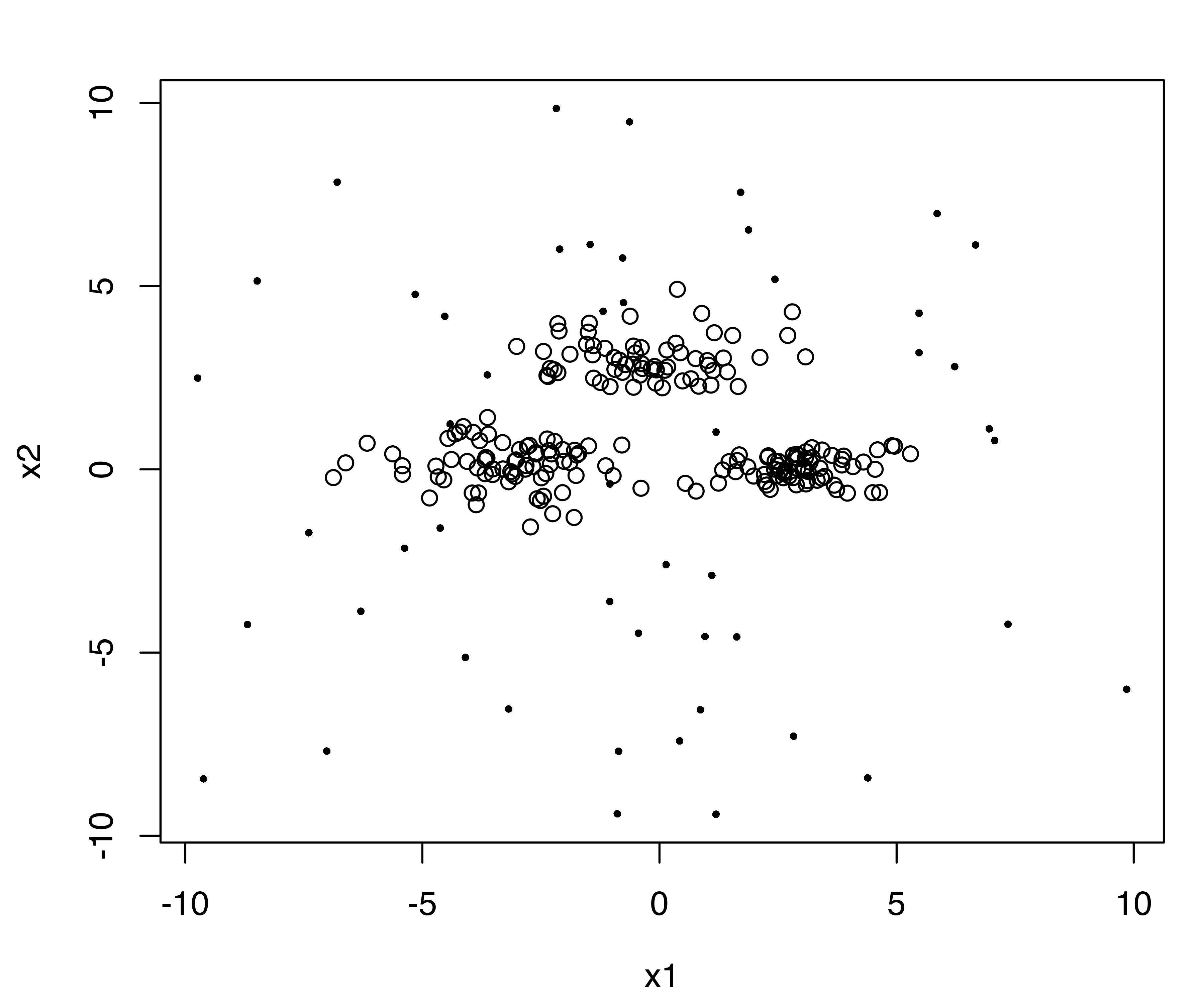
Consider the following simulated two-dimensional dataset with overlapping components as discussed in Baudry et al. (2010, sec. 4.1).
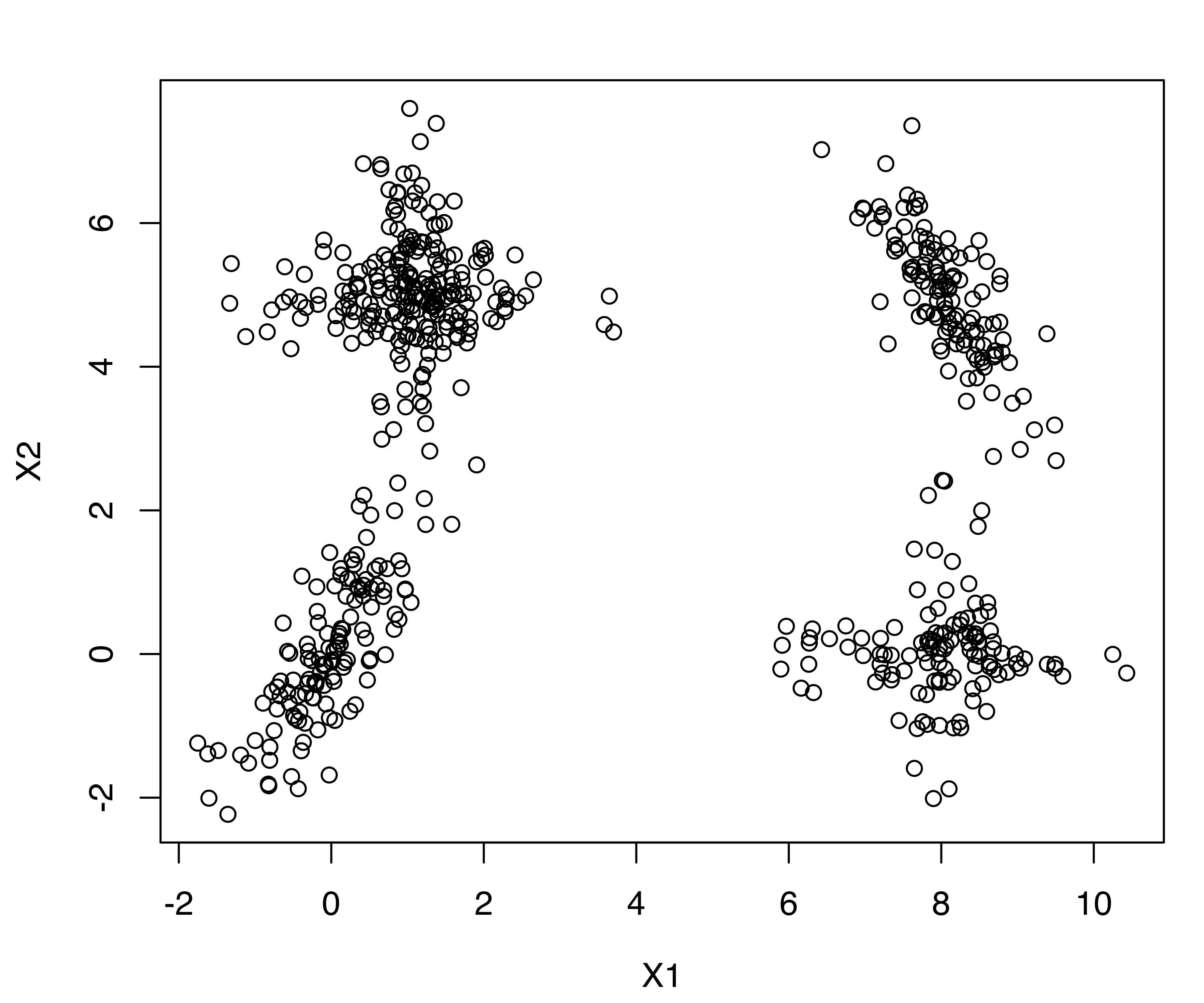
ex4.1 simulated dataset.
A sample of 600 observations was generated from a mixture of six Gaussian components, although it would be reasonable to conclude from the spatial distribution of the data that there are only four clusters. The data is shown in Figure 7.7. Two of the clusters are formed from overlapping axis-aligned components (diagonal covariance matrices), while the remaining two clusters are elliptical but not axis-aligned.
The estimated model maximizing the BIC criterion is the following:
mod_ex4.1 = Mclust(ex4.1)
summary(mod_ex4.1)
## ----------------------------------------------------
## Gaussian finite mixture model fitted by EM algorithm
## ----------------------------------------------------
##
## Mclust EEV (ellipsoidal, equal volume and shape) model with 6
## components:
##
##  log-likelihood   n df     BIC     ICL
##         -1957.8 600 25 -4075.5 -4248.4
##
## Clustering table:
##   1   2   3   4   5   6
##  78 122 121 107 132  40
The function clustCombi(), following the methodology described in Baudry et al. (2010), combines the mixture components hierarchically according to an entropy criterion. The estimated models with numbers of classes ranging from a single class to the number of components selected by BIC are returned as follows:
CLUSTCOMBI = clustCombi(mod_ex4.1)
summary(CLUSTCOMBI)
## ----------------------------------------------------
## Combining Gaussian mixture components for clustering
## ----------------------------------------------------
##
## Mclust model name: EEV
## Number of components: 6
##
## Combining steps:
##
## Step | Classes combined at this step | Class labels after this step
## -------|-------------------------------|-----------------------------
## 0 | --- | 1 2 3 4 5 6
## 1 | 3 & 4 | 1 2 3 5 6
## 2 | 1 & 6 | 1 2 3 5
## 3 | 3 & 5 | 1 2 3
## 4 | 1 & 2 | 1 3
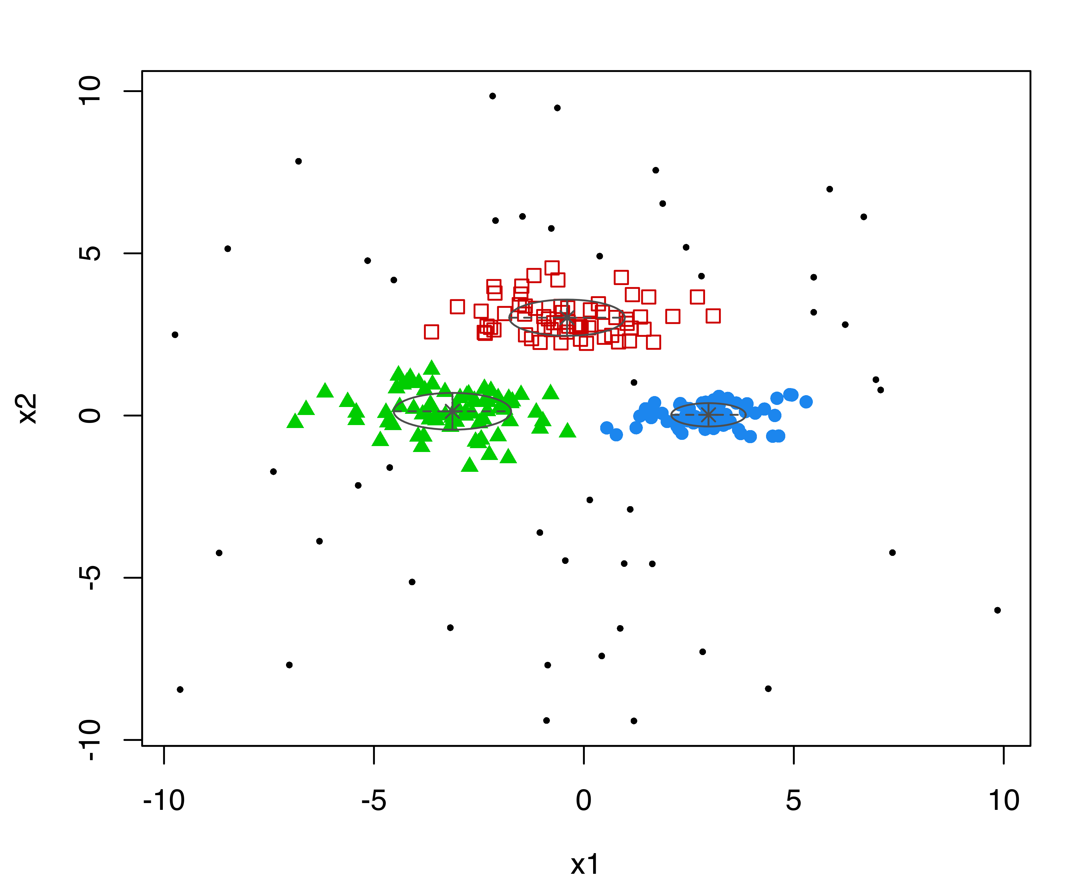
## 5 | 1 & 3 | 1The summary output shows the mixture model EEV with 6 components selected by the BIC criterion, followed by information describing the combining steps. The hierarchy of combined components can be displayed graphically as follows (see Figure 7.8):
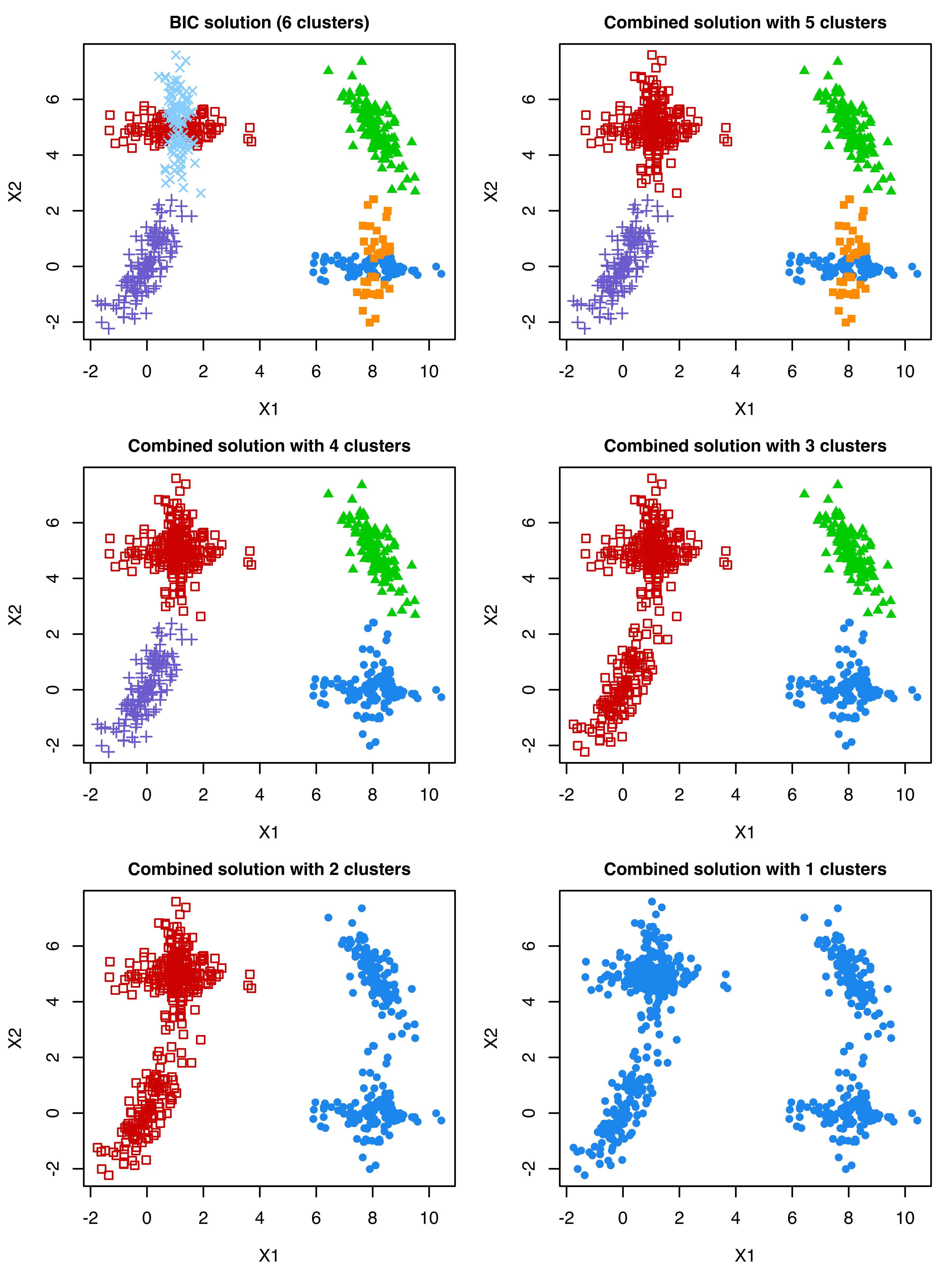
ex4.1 dataset.
The process of merging mixture components can also be represented using tree diagrams:
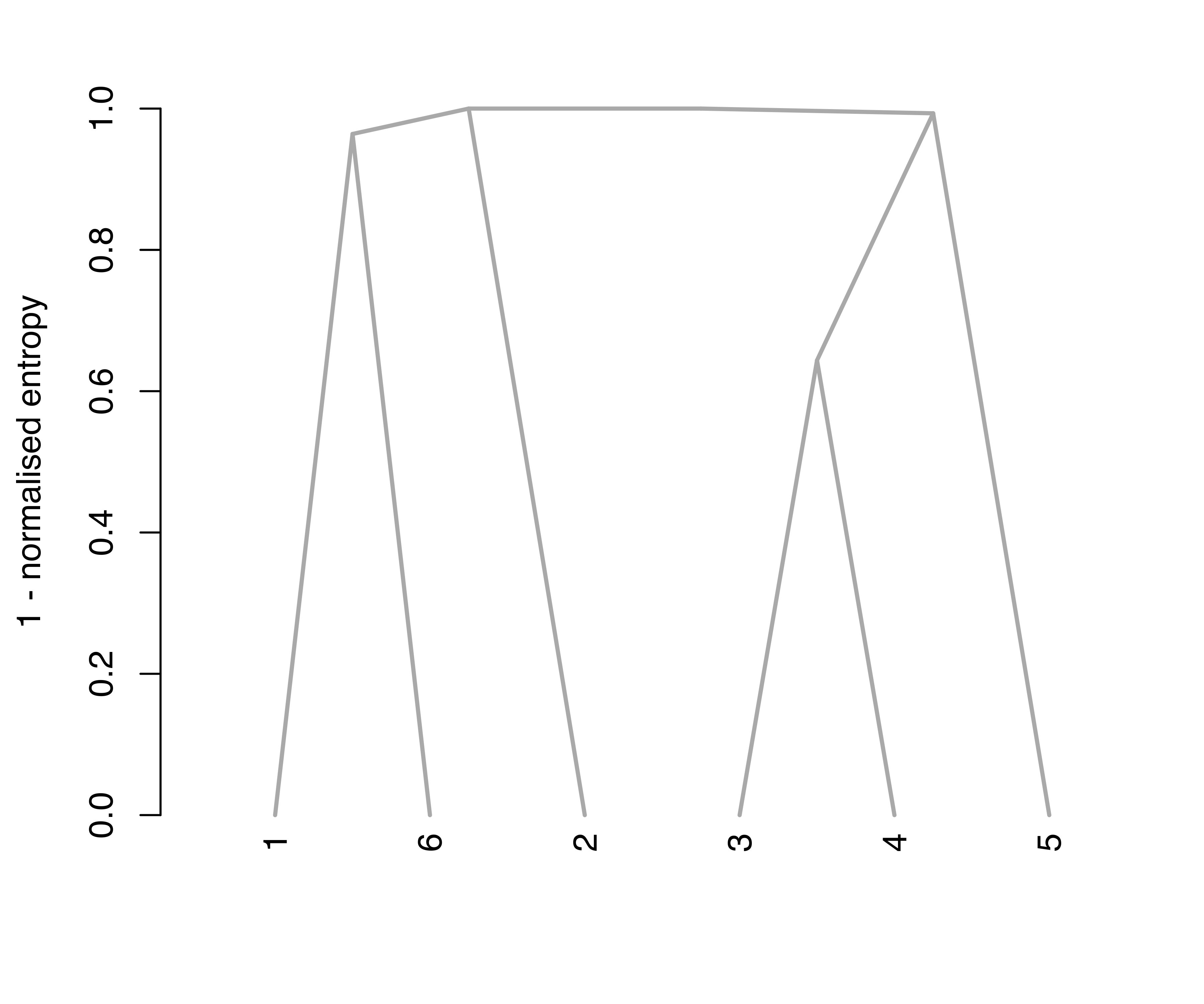
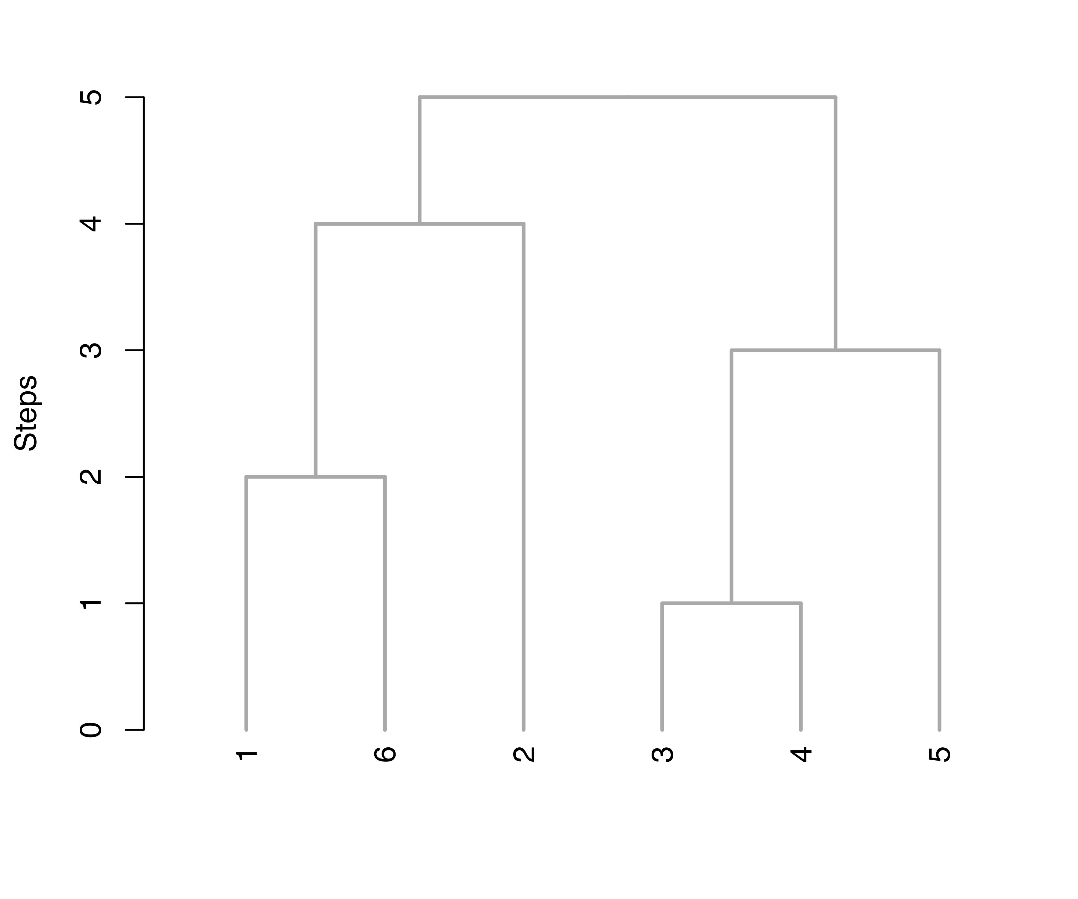
ex4.1 dataset.
Figure 7.9 (a) shows the resulting tree obtained using the default arguments, type = "triangle" and yaxis = "entropy". The first argument controls the type of dendrogram to plot; two options are available, namely, "triangle" and "rectangle". The second argument controls the quantity to appear on the \(y\)-axis; by default one minus the normalized entropy at each merging step is used. The option yaxis = "step" is also available to simply represent heights as successive steps, as shown in Figure 7.9 (b).
The clustering structures obtained with clustCombi() can be compared on substantive grounds or by selecting the number of clusters via a piecewise linear regression fit to the (possibly rescaled) “entropy plot”. An automatic procedure to help the user to select the optimal number of clusters using the above methodology based on the entropy is available through the function clustCombiOptim(). For example, the following code
optimClust = clustCombiOptim(CLUSTCOMBI, reg = 2, plot = TRUE)
str(optimClust)
## List of 3
## $ numClusters.combi: int 4
## $ z.combi : num [1:600, 1:4] 1.00 1.00 5.78e-04 1.85e-42 3.85e-35 ...
## $ cluster.combi : num [1:600] 1 1 2 3 3 4 4 3 3 2 ...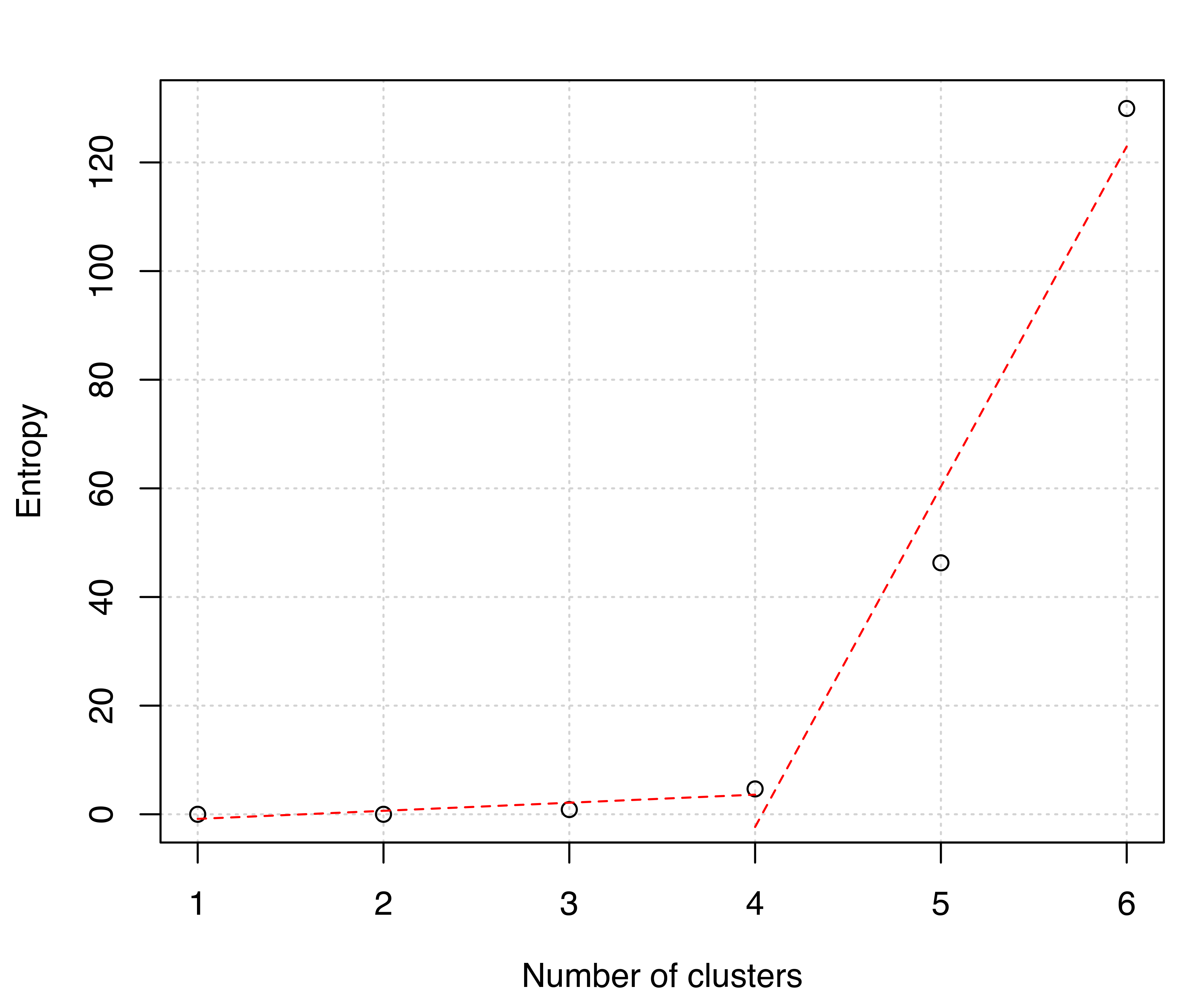
ex4.1 dataset.
produces the entropy plot in Figure 7.10 and returns a list containing the number of clusters (numClusters.combi), the probabilities (z.combi) obtained by summing posterior conditional probabilities over merged components, and the clustering labels (cluster.combi) obtained by merging the mixture components. The optional argument reg is used to specify the number of segments to use in the piecewise linear regression fit. Possible choices are 2 (the default, for a model with two segments or one change point) and 3 (for a model with three segments or two change points). The entropy plot clearly suggests a four-cluster solution.
7.3.2 Identifying Connected Components in GMMs
A limitation of approaches that successively combine mixture components is that, once merged, components cannot subsequently be reallocated to different clusters at a later stage of the algorithm.
Among the several definitions of “cluster” available in the literature, (Hartigan 1975, 205) proposed that “[…] clusters may be thought of as regions of high density separated from other such regions by regions of low density.” From this perspective, Scrucca (2016) defined high density clusters as connected components of density level sets. Starting with a density estimate obtained from a Gaussian finite mixture model, cluster cores — those data points which form the core of the clusters — are obtained from the connected components at a given density level. A mode function gives the number of connected components as the level is varied. Once cluster cores are identified, the remaining observations are allocated to those cluster cores for which the probability of cluster membership is the highest. Details are provided in Scrucca (2016) and implemented in the gmmhd() function available in mclust. A non-parametric variant proposed by Azzalini and Menardi (2014) is implemented in pdfCluster (Menardi and Azzalini 2022).
Example 7.6 Identifying high density clusters on the Old Faithful data
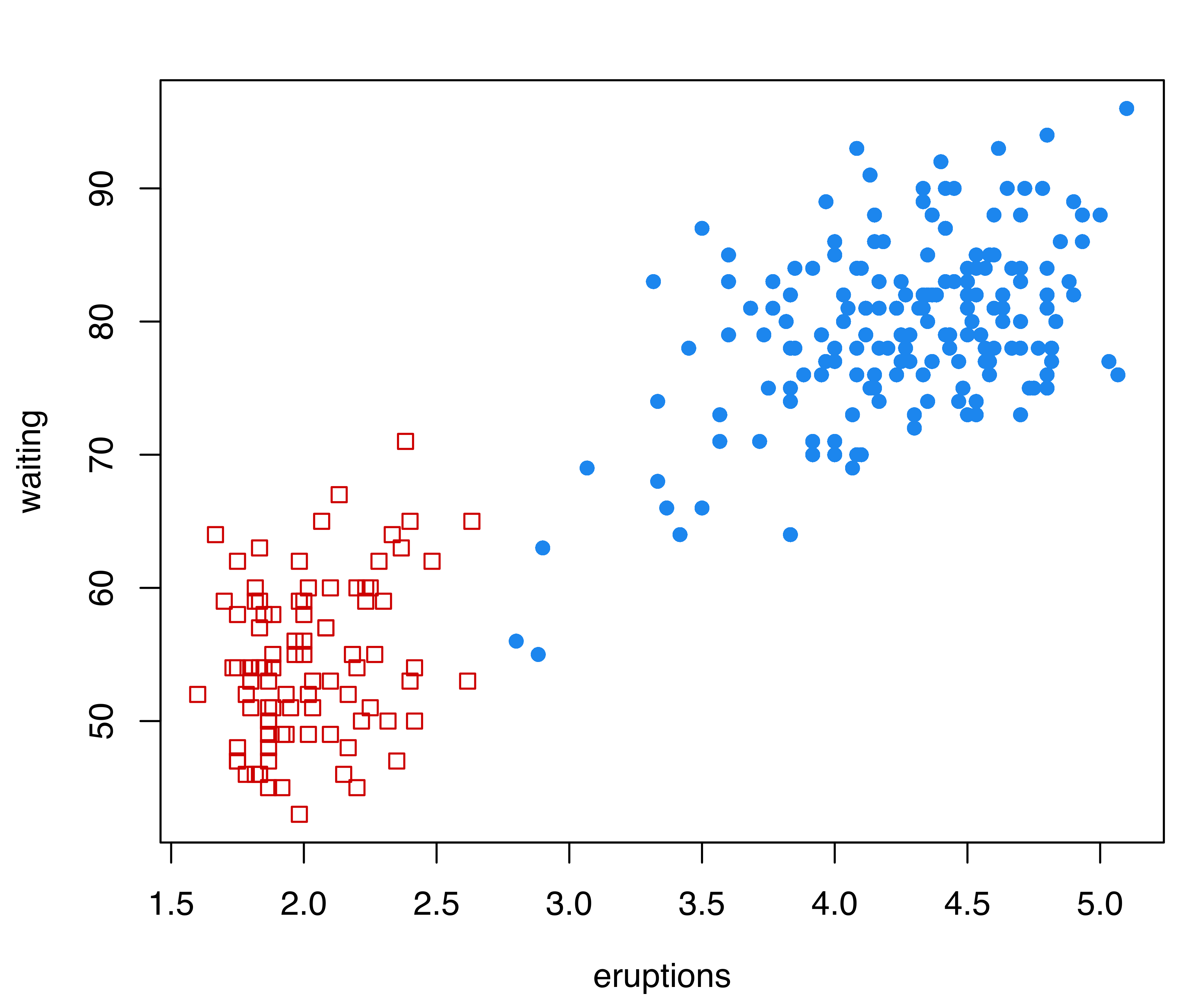
As a first example, consider the Old Faithful data described in Example 3.4.
data("faithful", package = "datasets")
mod = Mclust(faithful)
clPairs(faithful, mod$classification)
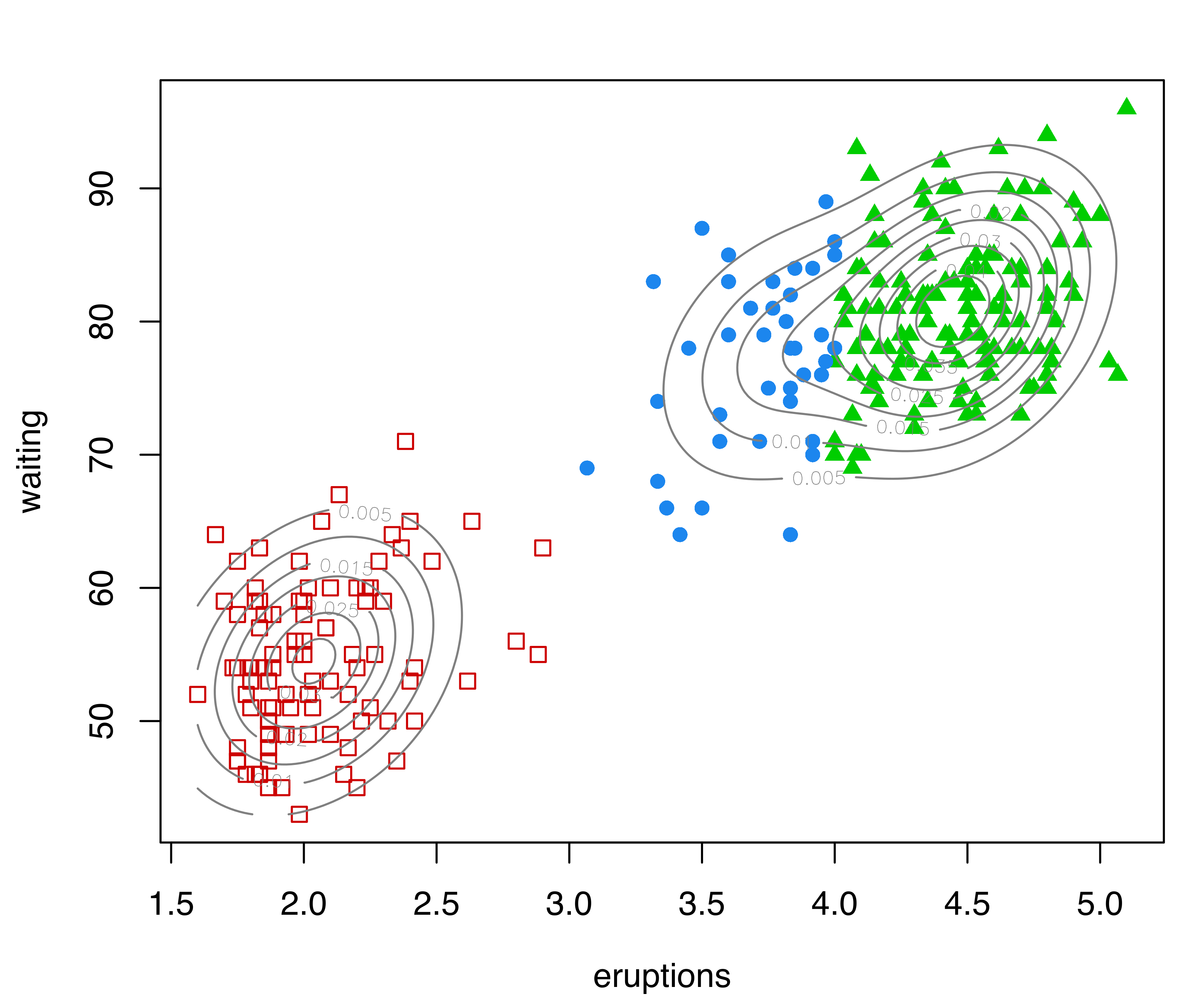
plot(as.densityMclust(mod), what = "density", add = TRUE)Figure 7.11 (a) shows the clustering partition obtained from the best estimated GMM according to BIC. The model selected is (EEE,3), a mixture of three components with common full covariance matrix. The portion of the data with high values for both waiting and eruptions is fitted with two Gaussian components. However, there appear to be two separate groups of points in the data as a whole, and the corresponding bivariate density estimate shown in Figure 7.11 (a) indicates the presence of two separate regions of high density.
The GMMHD approach (Scrucca 2016) briefly outlined at the beginning of this section is implemented in the gmmhd() function available in mclust. This function requires as input an object returned by Mclust() or densityMclust() as the initial GMM. Many other input parameters can be set, and the interested reader should consult the documentation available through help("gmmhd").
We apply the GMMHD algorithm to our example by invoking function gmmhd() and producing its summary output as follows:
GMMHD = gmmhd(mod)
summary(GMMHD)
## ---------------------------------------------------------
## GMM with high-density connected components for clustering
## ---------------------------------------------------------
##
## Initial model: Mclust (EEE,3)
##
## Cluster cores:
## 1 2 <NA>
## 166 91 15
##
## Final clustering:
## 1 2
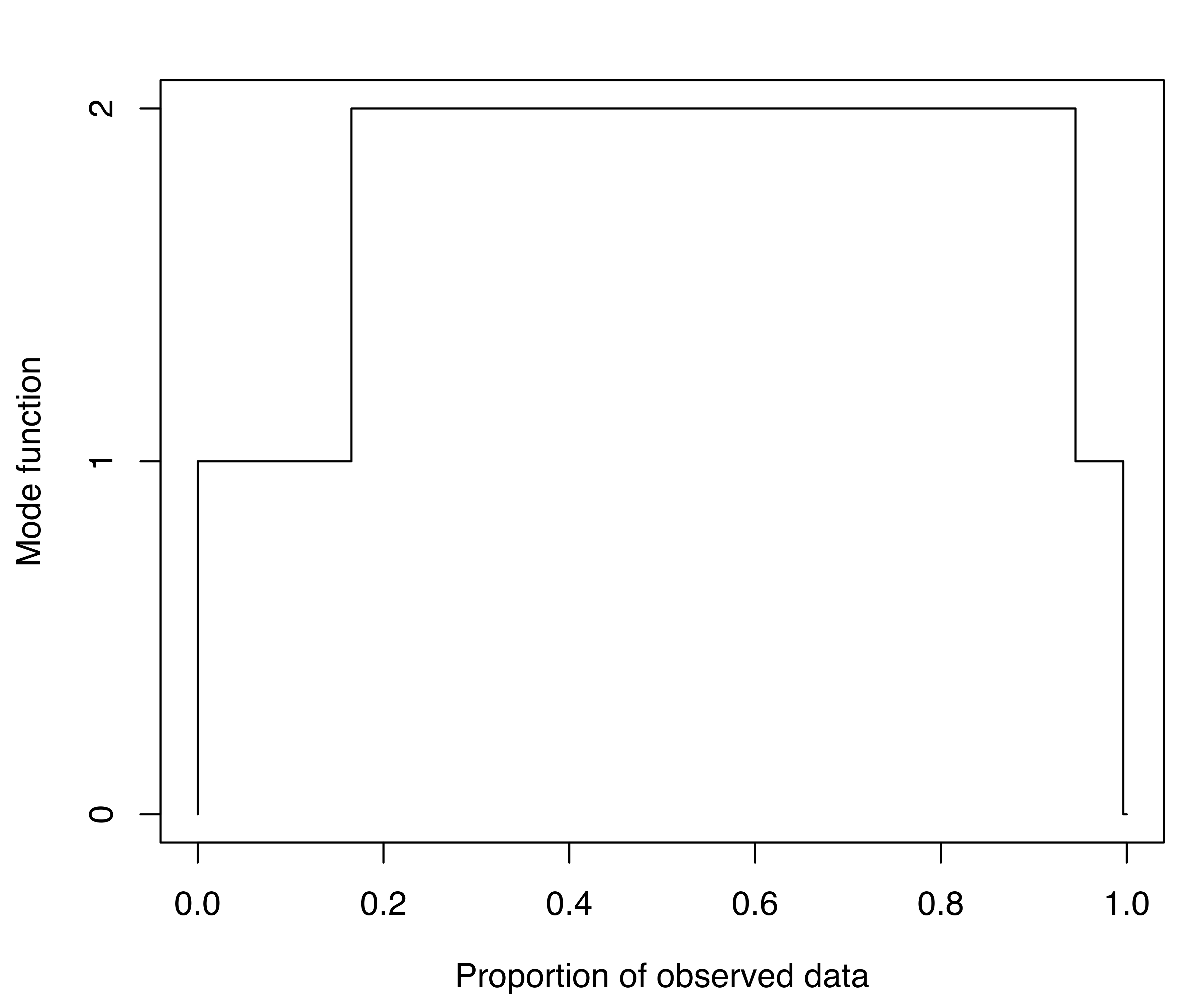
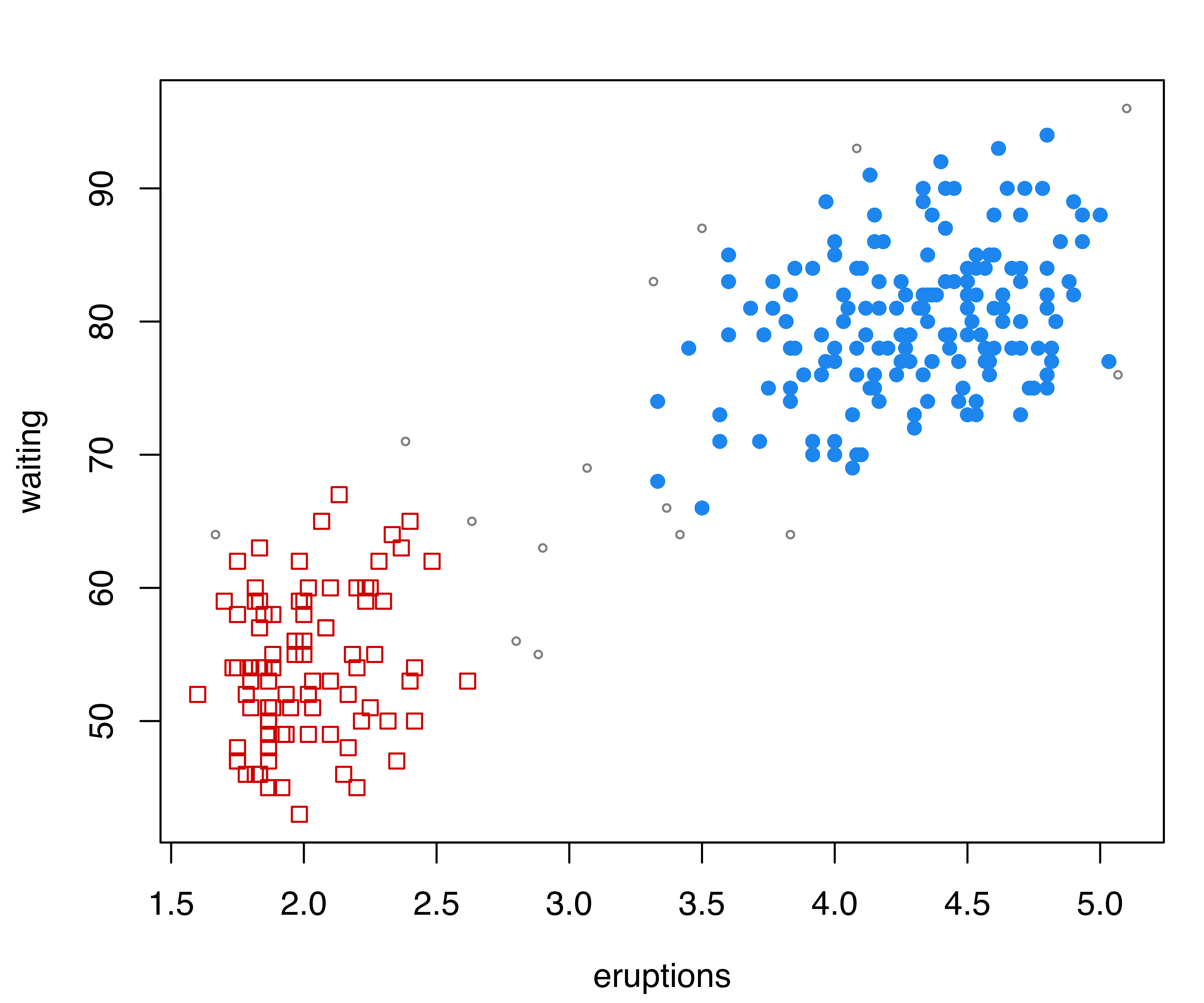
## 178 94Starting with the density estimate from the initial (EEE,3) Gaussian mixture model, gmmhd() computes the empirical mode function and the connected components at different density levels, which are then used to identify cluster cores. Figure 7.11 (b) plots the number of modes as a function of the proportion of data points above a threshold density level. There is a clear indication of a bimodal distribution. Figure 7.11 (c) shows the points assigned to the cluster cores, as well as the remaining data points not initially allocated.
The summary above shows that 166 and 91 observations have been assigned to the two cluster cores, and that 15 points were initially unlabeled. Figure 7.11 (d) shows the final clustering obtained after the unlabeled data have also been allocated to the cluster cores. Figure 7.11 (b)–Figure 7.11 (d) can be produced with the following commands:
Example 7.7 Simulated data {.unnumbered #sec-sim_data}
We now compare the results of the GMMHD procedure with the component combination methods of Section 7.3.1 on the simulated dataset from that section.
data("Baudry_etal_2010_JCGS_examples", package = "mclust")
mod = Mclust(ex4.1)
GMMHD = gmmhd(mod)
summary(GMMHD)
## ---------------------------------------------------------
## GMM with high-density connected components for clustering
## ---------------------------------------------------------
##
## Initial model:  Mclust (EEV,6)
##
## Cluster cores:
##    1    2    3    4 <NA>
##  100  116  111  206   67
##
## Final clustering:
##   1   2   3   4
## 118 133 122 227
optimClust = clustCombiOptim(clustCombi(mod), reg = 2)
table(GMMHD = GMMHD$cluster, CLUSTCOMBI = optimClust$cluster)
##      CLUSTCOMBI
## GMMHD   1   2   3   4
##     1 118   0   0   0
##     2   0   0   1 132
##     3   0 122   0   0
##     4   0   0 227   0
The GMMHD procedure identifies essentially the same four clusters as clustCombi(), with the exception of a single point on the edge of the two clusters on the left of graphs in Figure 7.8.
7.4 Simulation from Mixture Densities
Given the parameters of a mixture model, data can be simulated from that model for evaluation and verification. The mclust function sim() enables simulation from all of the structured GMMs supported. Besides the model, sim() allows a seed to be input for reproducibility.
Example 7.8 Simulating data from GMM estimated from the Old Faithful data
In the example below we simulate two different datasets of the same size as the faithful dataset from the model returned by Mclust():
The results can be plotted as follows (graphs not shown):
xlim = range(c(faithful[, 1], sim0[, 2], sim1[, 2]))
ylim = range(c(faithful[, 2], sim0[, 3], sim1[, 3]))
mclust2Dplot(data = sim0[, -1], parameters = mod$parameters,
             classification = sim0[, 1], xlim = xlim, ylim = ylim)
mclust2Dplot(data = sim1[, -1], parameters = mod$parameters,
             classification = sim1[, 1], xlim = xlim, ylim = ylim)
Note that sim() produces a dataset in which the first column is the true classification:
head(sim0)
##      group     x1     x2
## [1,]     1 4.1376 71.918
## [2,]     3 4.4703 77.198
## [3,]     3 4.5090 74.671
## [4,]     2 1.9596 49.380
## [5,]     1 4.0607 78.773
## [6,]     3 4.3597 82.190
7.5 Large Datasets
Gaussian mixture modeling may in practice be too slow to be applied directly to datasets having a large number of observations or cases. In order to extend the method to larger datasets, both Mclust() and mclustBIC() include a provision for using a subsample of the data in the initial hierarchical clustering phase before applying the EM algorithm to the full dataset. Other functions in the mclust package also have this feature. Some alternatives for handling large datasets are discussed by Wehrens et al. (2004) and C. Fraley, Raftery, and Wehrens (2005).
Starting with version 5.4 of mclust, a subsample of size specified by mclust.options("subset") is used in the initial hierarchical clustering phase. The default subset size is 2000. The subsampling can be removed by the command mclust.options(subset = Inf). The subset size can be specified for all the models in the current session through the subset argument to mclust.options(). Furthermore, the subsampling approach can also be implemented in the Mclust() function by setting initialization = list(subset = s), where s is a vector of logical values or numerical indices specifying the subset of data to be used in the initial hierarchical clustering phase.
Example 7.9 Clustering on a simulated large dataset
Consider a simulated dataset of \(n=10 000\) points from a three-component Gaussian mixture with common covariance matrix. First, we create a list, par, of the model parameters to be used in the simulation:
par = list(
  pro = c(0.5, 0.3, 0.2),
  mean = matrix(c(0, 0, 3, 3, -4, 1), nrow = 2, ncol = 3),
  variance = sigma2decomp(matrix(c(1, 0.6, 0.6, 1.5), nrow = 2, ncol = 2),
                          G = 3))
str(par)
## List of 3
## $ pro : num [1:3] 0.5 0.3 0.2
## $ mean : num [1:2, 1:3] 0 0 3 3 -4 1
## $ variance:List of 7
## ..$ sigma : num [1:2, 1:2, 1:3] 1 0.6 0.6 1.5 1 0.6 0.6 1.5 1 0.6 ...
## ..$ d : int 2
## ..$ modelName : chr "EEI"
## ..$ G : num 3
## ..$ scale : num 1.07
## ..$ shape : num [1:2] 1.78 0.562
## ..$ orientation: num [1:2, 1:2] 0.555 0.832 -0.832 0.555
We then simulate the data with the sim() function as described in Section 7.4:
sim = sim(modelName = "EEI", parameters = par, n = 10000, seed = 123)
cluster = sim[, 1]
x = sim[, 2:3]
The following code is used to fit GMMs with no subsampling, using the default subsampling, and a random sample of 1000 observations provided to the Mclust() function:
mclust.options(subset = Inf)  # no subsetting
system.time(mod1 = Mclust(x))
##    user  system elapsed
## 172.981   0.936 173.866
summary(mod1$BIC)
## Best BIC values:
##              EEI,3         EEE,3        EVI,3
## BIC      -76523.89 -76531.836803 -76541.59835
## BIC diff      0.00     -7.948006    -17.70955

mclust.options(subset = 2000)  # reset to default setting
system.time(mod2 = Mclust(x))
##  user  system elapsed
## 14.247   0.196  14.395
summary(mod2$BIC)
## Best BIC values:
##              EEI,3         EEE,3        EVI,3
## BIC      -76524.09 -76531.845624 -76541.89691
## BIC diff      0.00     -7.754063    -17.80535

s = sample(1:nrow(x), size = 1000)  # one-time subsetting
system.time(mod3 = Mclust(x, initialization = list(subset = s)))
##   user  system elapsed
## 12.091   0.146  12.197
summary(mod3$BIC)
## Best BIC values:
##              EEI,3         EEE,3        VEI,3
## BIC      -76524.17 -76532.043460 -76541.78983
## BIC diff      0.00     -7.874412    -17.62078
Function system.time() gives a rough indication of the computational effort associated without and with subsampling. In the latter case, using a random sample of 20% of the full set of observations, we have been able to obtain a \(10\) fold speedup, ending up with essentially the same final clustering model:
table(mod1$classification, mod2$classification)
##       1    2    3
##  1 5090    0    0
##  2    0    0 3007
##  3   10 1893    0
The same strategies that we have described for clustering very large datasets can also be used for classification. First, discriminant analysis with MclustDA() can be performed on a subset of the data. Then, the remaining data points can be classified (in reasonable sized blocks) using the associated predict() method.
7.6 High-Dimensional Data
Models in which the orientation is allowed to vary between components (EEV, VEV, EVV, and VVV), have \({\cal O}(d^2)\) parameters per cluster, where \(d\) is the dimension of the data (see Table 2.2 and Figure 2.3). For this reason, mclust may not work well or may otherwise be inefficient for these models when applied to high-dimensional data. It may still be possible to analyze such data with mclust by restricting to models with fewer parameters (spherical or diagonal models) or else by applying a dimension-reduction technique such as principal components analysis. Moreover, some of the more parsimonious models (spherical, diagonal, or fixed covariance) can be applied to datasets in which the number of observations is less than the data dimension.
7.7 Missing Data
At present, mclust has no direct provision for handling missing values in data. However, a function imputeData() for creating datasets with missing data imputations using the mix R package (Joseph L. Schafer 2022) has been added to the mclust package.
The algorithm used in imputeData() starts with a preliminary maximum likelihood estimation step to obtain model parameters for the subset of complete observations in the data. These are used as initial values for a data augmentation step for generating posterior draws of parameters via Markov Chain Monte Carlo. Finally, missing values are imputed with simulated values drawn from the predictive distribution of the missing data given the observed data and the simulated parameters.
Example 7.10 Imputation on the child development data
The stlouis dataset, available in the mix package, provides data from an observational study to assess the affects of parental psychological disorders on child development. Here we use imputeData() to fill in missing values in the continuous portion of the stlouis dataset; we remove the first 3 categorical variables, because mclust is intended for continuous variables.
data("stlouis", package = "mix")
x = data.frame(stlouis[, -(1:3)], row.names = NULL)
table(complete.cases(x))
##
## FALSE  TRUE
##    42    27
apply(x, 2, function(x) prop.table(table(complete.cases(x))))
##            R1      V1      R2      V2
## FALSE 0.30435 0.43478 0.23188 0.24638
## TRUE  0.69565 0.56522 0.76812 0.75362
The dataset contains only 27 complete cases out of 69 observations (39%). For each variable, the percentage of missing values ranges from 23% to 43%. The pattern of missing values can be displayed graphically using the following code (see Figure 7.12):
library("ggplot2")
df = data.frame(obs = rep(1:nrow(x), times = ncol(x)),
                var = rep(colnames(x), each = nrow(x)),
                missing = as.vector(is.na(x)))
ggplot(data = df, aes(x = var, y = obs)) +
  geom_tile(aes(fill = missing)) +
  scale_fill_manual(values = c("lightgrey", "black")) +
  labs(x = "Variables", y = "Observations") +
  theme_minimal() +
  theme(axis.text.x = element_text(margin = margin(b = 10))) +
  theme(axis.ticks.y = element_blank()) +
  theme(axis.text.y = element_blank())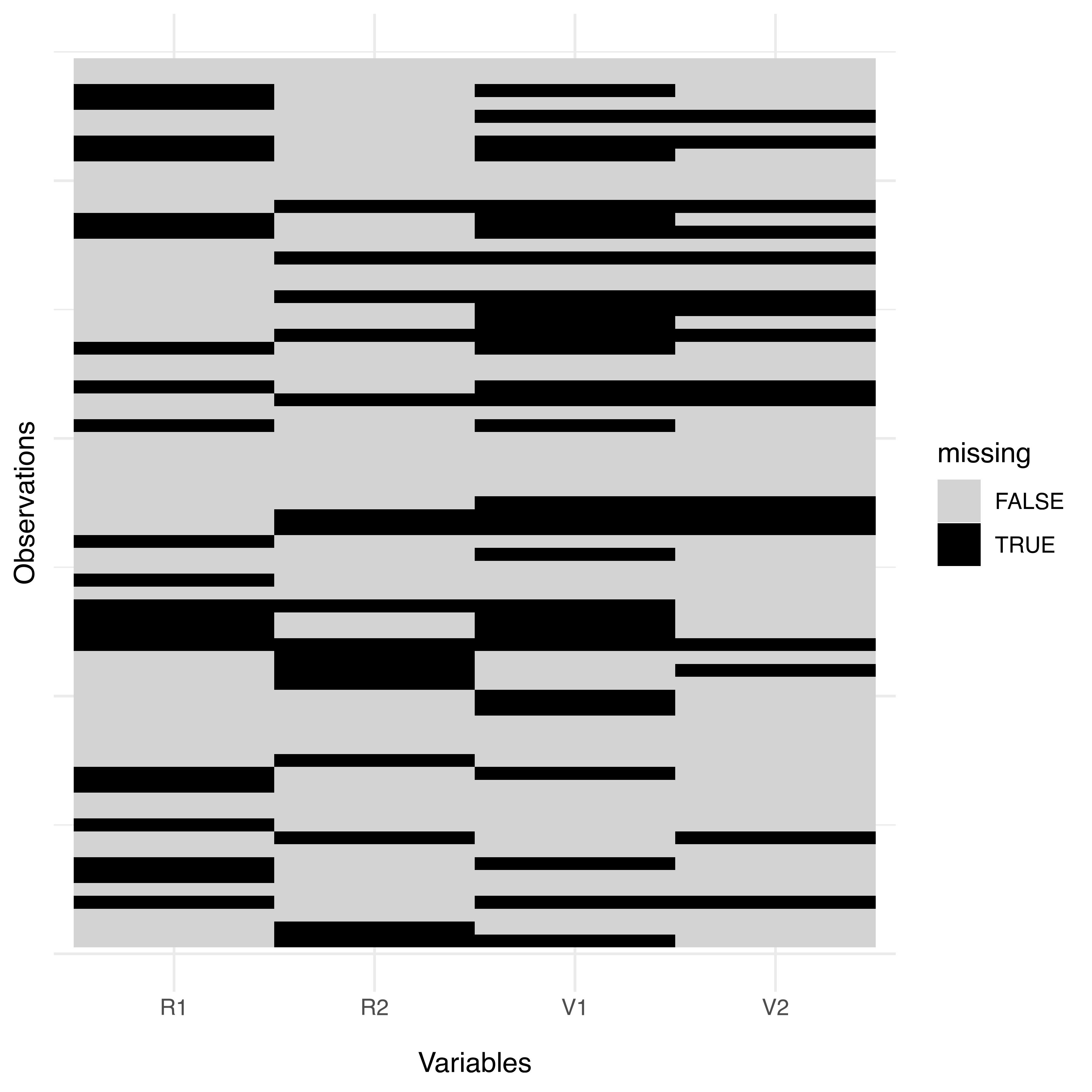
stlouis dataset.
A single imputation of simulated values drawn from the predictive distribution of the missing data is easily obtained as
ximp = imputeData(x, seed = 123)Note that the values obtained for the missing entries will vary depending on the random number seed set as argument in the imputeData() function call. By default, a randomly chosen seed is used.
Missing data imputations can be visualized with the function imputePairs() as follows:
imputePairs(x, ximp)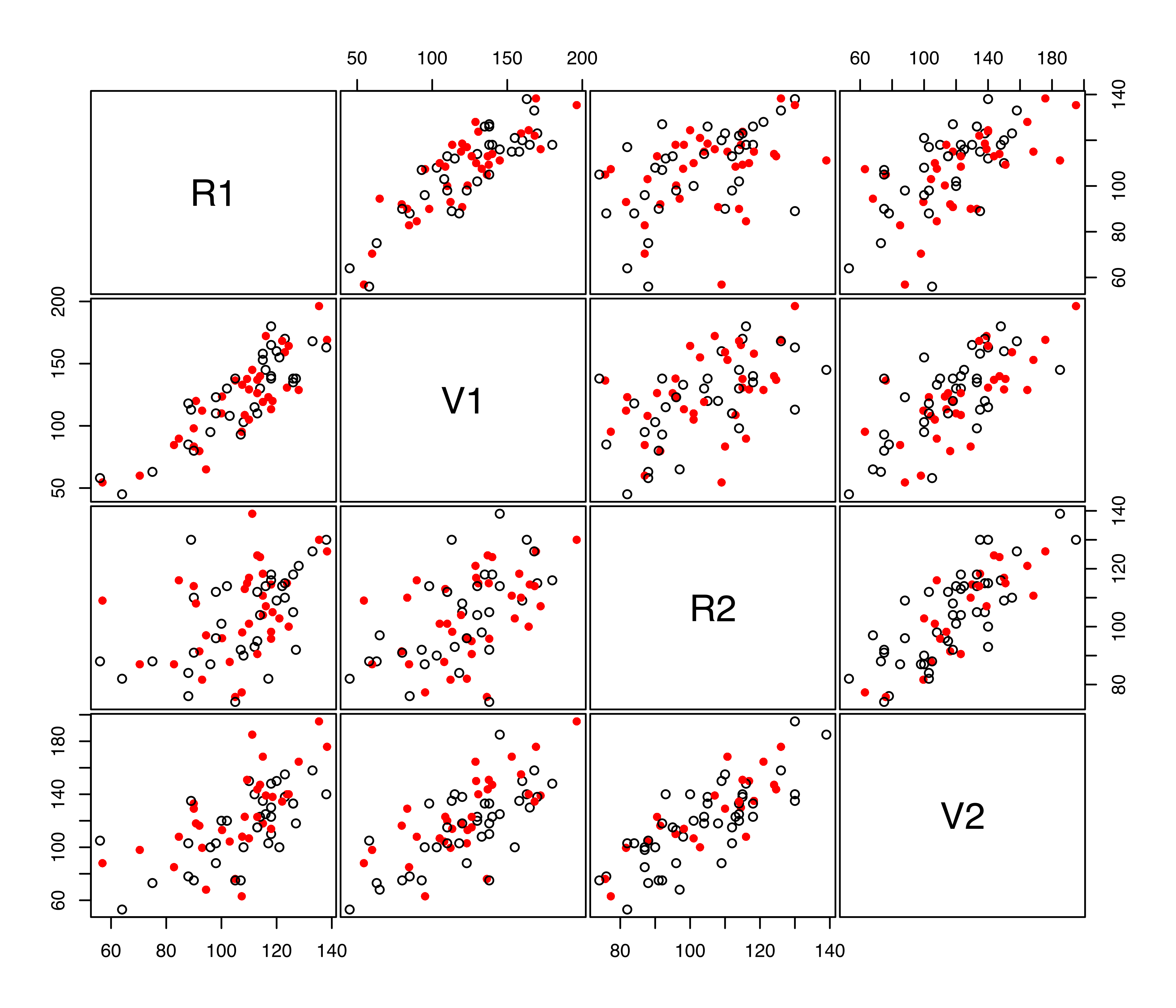
imputeData() to the continuous variables in the stlouis dataset. The open black circles correspond to non-missing data, while the filled red circles correspond to imputed missing values.
The corresponding pairs plot is shown in Figure 7.13.
It is usually desirable to combine multiple imputations in analyses involving missing data. See Joseph L. Schafer (1997), Little and Rubin (2002), and van Buuren and Groothuis-Oudshoorn (2011) for details and references on multiple imputation. Besides mix, R packages for handling missing data include Amelia (Honaker, King, and Blackwell 2011) and mice (van Buuren 2012).
Example 7.11 Clustering with missing values on the Iris data
We now illustrate a model-based clustering analysis in the presence of missing values. Consider the iris data, and suppose that we want to fit a three-component model with common full covariance matrix. The model using the full set of observations is obtained as follows:
x = as.matrix(iris[, 1:4])
mod = Mclust(x, G = 3, modelNames = "EEE")
table(iris$Species, mod$classification)
##
##               1  2  3
##   setosa     50  0  0
##   versicolor  0 48  2
##   virginica   0  1 49
adjustedRandIndex(iris$Species, mod$classification)
## [1] 0.94101
mod$parameters$mean  # component means
##               [,1]   [,2]   [,3]
## Sepal.Length 5.006 5.9426 6.5749
## Sepal.Width  3.428 2.7607 2.9811
## Petal.Length 1.462 4.2596 5.5394
## Petal.Width  0.246 1.3194 2.0254
Here we assume that the interest is in the final clustering partition and in the corresponding component means. Other mixture parameters, such as mixing probabilities and (co)variances, can be dealt with analogously.
Now, let us randomly designate 10% of the data values as missing:
The last command shows that 100 out of 150 observations have no missing values. We can use multiple imputation to create nImp complete datasets by replacing the missing values with plausible data values. Then, an (EEE,3) clustering model is fitted to each of these datasets, and the results are pooled to get the final estimates.
A couple of issues should be mentioned. First, a well-known issue of finite mixture modeling is nonidentifiability of the components due to invariance to relabeling. This is solved in the code below using matchCluster(), which takes the first clustering result as a template for adjusting the labeling of the successive clusters. The adjusted ordering is also used for matching the other estimated parameters.
A second issue is related to how pooling of results is carried out at the end of the imputation procedure. For the clustering labels, the majority vote rule is used as implemented in function majorityVote(), whereas a simple average of estimates is calculated for pooling results for the mean parameters.
nImp  = 100
muImp = array(NA, c(ncol(x), 3, nImp))
clImp = array(NA, c(nrow(x), nImp))
for(i in 1:nImp)
{
  xImp = imputeData(x, verbose = FALSE)
  modImp = Mclust(xImp, G = 3, modelNames = "EEE", verbose = FALSE)
  if (i == 1) clImp[, i] = modImp$classification
  mcl = matchCluster(clImp[, 1], modImp$classification)
  clImp[, i]  = mcl$cluster
  muImp[, , i] = modImp$parameters$mean[, mcl$ord]
}

# majority rule
cl = apply(clImp, 1, function(x) majorityVote(x)$majority)
table(iris$Species, cl)
##             cl
##               1  2  3
##   setosa     50  0  0
##   versicolor  0 49  1
##   virginica   0  5 45
adjustedRandIndex(iris$Species, cl)
## [1] 0.88579

# pooled estimate of cluster means
apply(muImp, 1:2, mean)
##         [,1]   [,2]   [,3]
## [1,] 4.99885 5.9388 6.5667
## [2,] 3.44614 2.7684 2.9675
## [3,] 1.48357 4.2783 5.5453
## [4,] 0.25557 1.3333 2.0267
It is interesting to note that both the final clustering obtained by majority vote and cluster means obtained by pooling results from imputed datasets are quite close to those obtained on the original dataset.