5 Model-Based Density Estimation
\[ \DeclareMathOperator{\Real}{\mathbb{R}} \DeclareMathOperator{\Proj}{\text{P}} \DeclareMathOperator{\Exp}{\text{E}} \DeclareMathOperator{\Var}{\text{Var}} \DeclareMathOperator{\var}{\text{var}} \DeclareMathOperator{\sd}{\text{sd}} \DeclareMathOperator{\cov}{\text{cov}} \DeclareMathOperator{\cor}{\text{cor}} \DeclareMathOperator{\range}{\text{range}} \DeclareMathOperator{\rank}{\text{rank}} \DeclareMathOperator{\ind}{\perp\hspace*{-1.1ex}\perp} \DeclareMathOperator{\CE}{\text{CE}} \DeclareMathOperator{\BS}{\text{BS}} \DeclareMathOperator{\ECM}{\text{ECM}} \DeclareMathOperator{\BSS}{\text{BSS}} \DeclareMathOperator{\WSS}{\text{WSS}} \DeclareMathOperator{\TSS}{\text{TSS}} \DeclareMathOperator{\BIC}{\text{BIC}} \DeclareMathOperator{\ICL}{\text{ICL}} \DeclareMathOperator{\CV}{\text{CV}} \DeclareMathOperator{\diag}{\text{diag}} \DeclareMathOperator{\se}{\text{se}} \DeclareMathOperator{\Cov}{\text{Cov}} \DeclareMathOperator{\boot}{\text{boot}} \DeclareMathOperator{\LRTS}{\text{LRTS}} \DeclareMathOperator{\Model}{\mathcal{M}} \DeclareMathOperator*{\argmin}{arg\min} \DeclareMathOperator*{\argmax}{arg\max} \DeclareMathOperator{\vech}{vech} \DeclareMathOperator{\tr}{tr} \]
Density estimation plays an important role in both applied data analysis and theoretical research in statistics. Finite mixture models provide a flexible semiparametric methodology for density estimation, where the unknown density can be regarded as a convex linear combination of one or more probability density functions. This chapter illustrates data examples where Gaussian mixtures are used for model-based univariate and multivariate density estimation.
5.1 Density Estimation
Density estimation is a valuable tool for summarizing data distributions. A good density estimate can reveal important characteristics of the data as well as provide a useful exploratory tool. Broadly speaking, three alternative approaches can be distinguished: parametric density estimation, nonparametric density estimation, and semiparametric density estimation via finite mixture modeling.
In the parametric approach, a distribution is assumed for the density with unknown parameters that are estimated by fitting a parametric function to the observed data. In the nonparametric approach, no density function is assumed a priori; rather, its form is completely determined by the data. Histograms and kernel density estimation (KDE) are two popular methods that belong to this class, and in both the number of parameters generally grows with the sample size and dimensionality of the dataset (Silverman 1998; Scott 2009). For univariate data, functions hist() and density() are available in base R for nonparametric density estimation, and several other packages, such as KernSmooth (Wand 2021), ks (Duong 2022), and sm (A. Bowman et al. 2022), either include functionality or are devoted to this approach. However, extension to higher dimensions is less well established.
Finite mixture models provide a flexible semiparametric methodology for density estimation. In this approach, the unknown density is expressed as a convex linear combination of one or more probability density functions. The Gaussian mixture model (GMM), which assumes the Gaussian distribution for the underlying component densities, is a popular choice in this class of methods. GMMs can approximate any continuous density with arbitrary accuracy, provided the model has a sufficient number of components (Ferguson 1983; Marron and Wand 1992; Escobar and West 1995; Roeder and Wasserman 1997; Frühwirth-Schnatter 2006). The number of parameters increases with the number of components, as well as with the dimensionality of the data except in the simplest case.
Advantages of the Gaussian mixture modeling in this context include:
No need to specify tuning parameters, such as the number of bins and the origin for histograms, or the bandwidth for kernel density estimation;
Efficient even for multidimensional data;
Maximum likelihood estimates are available.
Disadvantages of the Gaussian mixture modeling approach include:
Estimation via the EM algorithm may be slow and requires good starting values;
Bias-variance trade-off: many GMM components may be needed for approximating a distribution, increasing the variance of the estimates, while more parsimonious models reduce the variability but may introduce some bias.
The number of components to include is not known in advance.
5.2 Finite Mixture Modeling for Density Estimation with mclust
Consider a vector of random variables \(\boldsymbol{x}\) taking values in the sample space \(\Real{^d}\) with \(d \ge 1\), and assume that the probability density function can be written as a finite mixture density of \(G\) components as in equation Equation 2.1. The model adopted in this chapter assumes a Gaussian distribution for each component density, so the density of \(\boldsymbol{x}\) can be written as \[ f(\boldsymbol{x}) = \sum_{k=1}^G \pi_k \phi(\boldsymbol{x}; \boldsymbol{\mu}_k, \boldsymbol{\Sigma}_k), \] where \(\phi(\cdot)\) is the (multivariate) Gaussian density with mean \(\boldsymbol{\mu}_k\), covariance matrix \(\boldsymbol{\Sigma}_k\), and mixing weight \(\pi_k\) for component \(k\) (\(\pi_k > 0\), \(\sum_{k=1}^G \pi_k = 1\)), with \(k=1,\dots,G\). This is essentially a GMM of the form given in Equation 2.3.
Gaussian finite mixture modeling is a general strategy for density estimation. Nonparametric kernel density estimation (KDE) can be viewed as a mixture of \(G = n\) components with uniform weights: \(\pi_k = 1/n\) (Titterington, Smith, and Makov 1985, 28–29). Compared to KDE, finite mixture modeling typically uses a smaller number of components and hence fewer parameters. Conversely, compared to fully parametric density estimation, finite mixture modeling has the potential advantage of using more parameters and so introducing less estimation bias.
Mixture modeling also has its drawbacks, such as increased learning complexity and the need for iterative numerical procedures (such as the EM algorithm) for estimation. In certain cases there can also be identifiability issues (see Section 2.1.2).
mclust provides a simple interface to Gaussian mixture models for univariate and multivariate density estimation through the densityMclust() function. Available arguments and functionalities are analogous to those described in Section 3.2 for the Mclust() function in the clustering case. Several examples of its usage are provided in the following sections.
5.3 Univariate Density Estimation
Example 5.1 Density estimation of Hidalgo stamp data
Izenman and Sommer (1988) considered fitting a Gaussian mixture to the distribution of the thickness of stamps in the 1872 Hidalgo stamp issue of Mexico. The dataset is available in R package multimode (Ameijeiras-Alonso et al. 2021).
A density estimate based on GMMs can be obtained in mclust with the function densityMclust(), which also produces a plot of the estimated density:
dens = densityMclust(Thickness)The plot can be suppressed by setting the optional argument plot = FALSE. A summary can be obtained as follows:
summary(dens, parameters = TRUE)
## -------------------------------------------------------
## Density estimation via Gaussian finite mixture modeling
## -------------------------------------------------------
##
## Mclust V (univariate, unequal variance) model with 3 components:
##
##  log-likelihood   n df    BIC    ICL
##          1516.6 485  8 2983.8 2890.9
##
## Mixing probabilities:
##       1       2       3
## 0.26535 0.30179 0.43286
##
## Means:
##        1        2        3
## 0.072145 0.079346 0.099189
##
## Variances:
##            1            2            3
## 0.0000047749 0.0000031193 0.0001886446
This summary output shows that the estimated model selected by BIC is a three-component mixture with different variances (V,3), and gives the values of the estimated parameters.
The density estimate can also be displayed with the associated plot() method. For instance, Figure 5.1 shows the estimated density drawn over a histogram of the observed data. The latter is added by providing the optional argument data and specifying the break points between histogram bars (in the base R hist() function) by setting the argument breaks:
br = seq(min(Thickness), max(Thickness), length.out = 21)
plot(dens, what = "density", data = Thickness, breaks = br)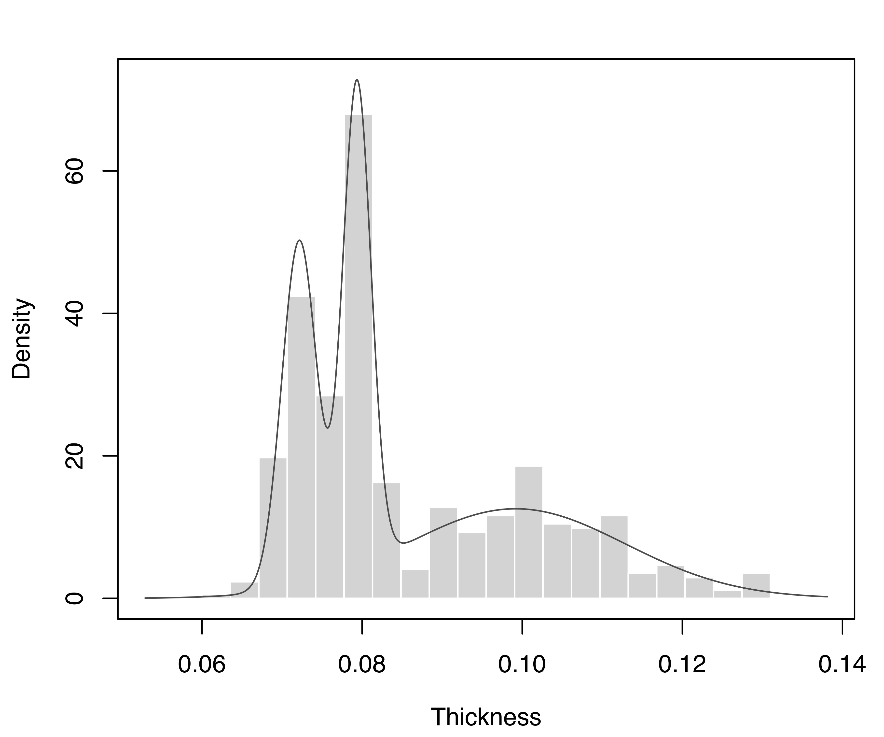
stamps1 dataset, with the GMM density estimate superimposed.
Three modes are clearly visible in the plot. These appear at the values of the mean of each mixture component: one component with larger mean and dispersion of stamp thickness, and two components having thinner and less variable stamps:
with(dens$parameters,
     data.frame(mean = mean,
                sd = sqrt(variance$sigmasq),
                CoefVar = sqrt(variance$sigmasq)/mean*100))
##       mean        sd CoefVar
## 1 0.072145 0.0021852  3.0288
## 2 0.079346 0.0017662  2.2259
## 3 0.099189 0.0137348 13.8470
A predict() method is associated with objects of class "densityMclust", for computing either the overall density (what = "dens", the default), or the individual (unweighted) mixture component densities (what = "cdens") at specified data points. Densities are returned on the logarithmic scale if we set logarithm = TRUE. For instance:
x = c(0.07, 0.08, 0.1, 0.12)
predict(dens, newdata = x, what = "dens")
## [1] 31.2340 68.4716 12.5509  3.9895
predict(dens, newdata = x, logarithm = TRUE)
## [1] 3.4415 4.2264 2.5298 1.3837
predict(dens, newdata = x, what = "cdens")
##                1           2       3
## [1,]  1.1275e+02  1.8734e-04  3.0362
## [2,]  2.8553e-01  2.1093e+02 10.9450
## [3,]  9.4735e-34  4.5561e-28 28.9956
## [4,] 1.3055e-102 2.0026e-113  9.2166
The matrix of posterior conditional probabilities is obtained by specifying what = "z":
predict(dens, newdata = x, what = "z")
##                1           2        3
## [1,]  9.5792e-01  1.8102e-06 0.042077
## [2,]  1.1065e-03  9.2970e-01 0.069191
## [3,]  2.0029e-35  1.0955e-29 1.000000
## [4,] 8.6832e-104 1.5149e-114 1.000000
The stamps1 dataset contains additional information that can be used to shed light on the selected model. In particular, thickness measurements can be grouped according to the year of consignment: the first 289 stamps refer to the 1872 issue and the remaining 196 stamps to the years 1873–1874. We may draw a (suitably scaled) histogram for each year-of-consignment and then add the estimated component densities as follows:
Year = stamps1$year
table(Year)
## Year
##      1872 1873-1874
##       289       196
h1 = hist(Thickness[Year == "1872"], breaks = br, plot = FALSE)
h1$density = h1$density*prop.table(table(Year))[1]
h2 = hist(Thickness[Year == "1873-1874"], breaks = br, plot = FALSE)
h2$density = h2$density*prop.table(table(Year))[2]
x = seq(min(Thickness)-diff(range(Thickness))/10,
         max(Thickness)+diff(range(Thickness))/10, length = 200)
cdens = predict(dens, x, what = "cdens")
cdens = sweep(cdens, 2, dens$parameters$pro, "*")
col = adjustcolor(mclust.options("classPlotColors")[1:2], alpha = 0.3)
ylim = range(h1$density, h2$density, cdens)
plot(h1, xlab = "Thickness", freq = FALSE, main = "", border = "white",
col = col[1], xlim = range(x), ylim = ylim)
plot(h2, add = TRUE, freq = FALSE, border = "white", col = col[2])
matplot(x, cdens, type = "l", lwd = 1, lty = 1, col = 1, add = TRUE)
box()
legend("topright", legend = levels(Year), col = col, pch = 15, inset = 0.02,
       title = "Overprinted years:", title.adj = 0.2)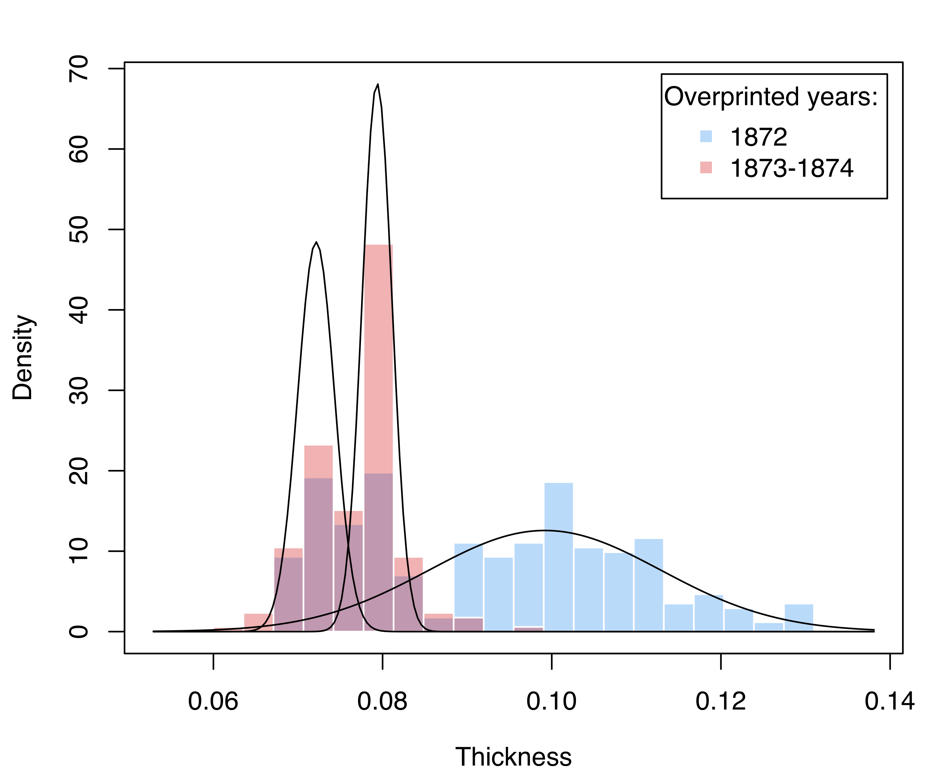
stamps1 dataset, with mixture component-density estimates superimposed.
The result is shown in Figure 5.2. Stamps from 1872 show a two-part distribution, with one component corresponding to the largest thickness, and one whose distribution essentially overlaps with the bimodal distribution of stamps for the years 1873–1874.
Example 5.2 Density estimation of acidity data
Consider the distribution of an acidity index measured on a sample of 155 lakes in the Northeastern United States. The data have been analyzed on the logarithmic scale using mixtures of normal distributions by Richardson and Green (1997) and (McLachlan and Peel 2000, sec. 6.6.2). The dataset is included in the CRAN package BNPdensity (Arbel et al. 2021; Barrios et al. 2021) and can be accessed as follows:
data("acidity", package = "BNPdensity")Using BIC as the model selection criterion, the “best” estimated model with respect to both the variance structure and the number of components can be obtained as follows:
summary(mclustBIC(acidity), k = 5)
## Best BIC values:
##              E,2       V,3       V,2       E,5      E,3
## BIC      -392.07 -397.9108 -399.6945 -400.6745 -402.183
## BIC diff    0.00   -5.8385   -7.6222   -8.6022  -10.111
BIC supports the two-component model with equal variance across the components (E,2). This model can be estimated as follows:
dens_E2 = densityMclust(acidity, G = 2, modelNames = "E")
summary(dens_E2, parameters = TRUE)
## -------------------------------------------------------
## Density estimation via Gaussian finite mixture modeling
## -------------------------------------------------------
##
## Mclust E (univariate, equal variance) model with 2 components:
##
##  log-likelihood   n df     BIC     ICL
##         -185.95 155  4 -392.07 -398.56
##
## Mixing probabilities:
##       1       2
## 0.62336 0.37664
##
## Means:
##      1      2
## 4.3709 6.3202
##
## Variances:
##       1       2
## 0.18637 0.18637
Next, we provisionally assume a GMM with unequal variances and decide the number of mixture components via the bootstrap LRT discussed in Section 2.3.2 instead of the BIC:
mclustBootstrapLRT(acidity, modelName = "V")
## -------------------------------------------------------------
## Bootstrap sequential LRT for the number of mixture components
## -------------------------------------------------------------
## Model        = V
## Replications = 999
##             LRTS bootstrap p-value
## 1 vs 2   77.0933             0.001
## 2 vs 3   16.9140             0.005
## 3 vs 4    5.1838             0.301
LRT suggests a three-component Gaussian mixture (V,3), which was a fairly close second-best fit according to BIC. This (V,3) model can be estimated as follows:
dens_V3 = densityMclust(acidity, G = 3, modelNames = "V")
summary(dens_V3, parameters = TRUE)
## -------------------------------------------------------
## Density estimation via Gaussian finite mixture modeling
## -------------------------------------------------------
##
## Mclust V (univariate, unequal variance) model with 3 components:
##
##  log-likelihood   n df     BIC     ICL
##         -178.78 155  8 -397.91 -458.86
##
## Mixing probabilities:
##       1       2       3
## 0.34061 0.31406 0.34534
##
## Means:
##      1      2      3
## 4.2040 4.6796 6.3809
##
## Variances:
##        1        2        3
## 0.044195 0.338309 0.178276
The parameter estimates for the GMMs are available from the summary() output, and the corresponding density functions can be plotted with the following code:
plot(dens_E2, what = "density",
     ylim = c(0, max(dens_E2$density, dens_V3$density)))
rug(acidity)
plot(dens_V3, what = "density",
     ylim = c(0, max(dens_E2$density, dens_V3$density)))
rug(acidity)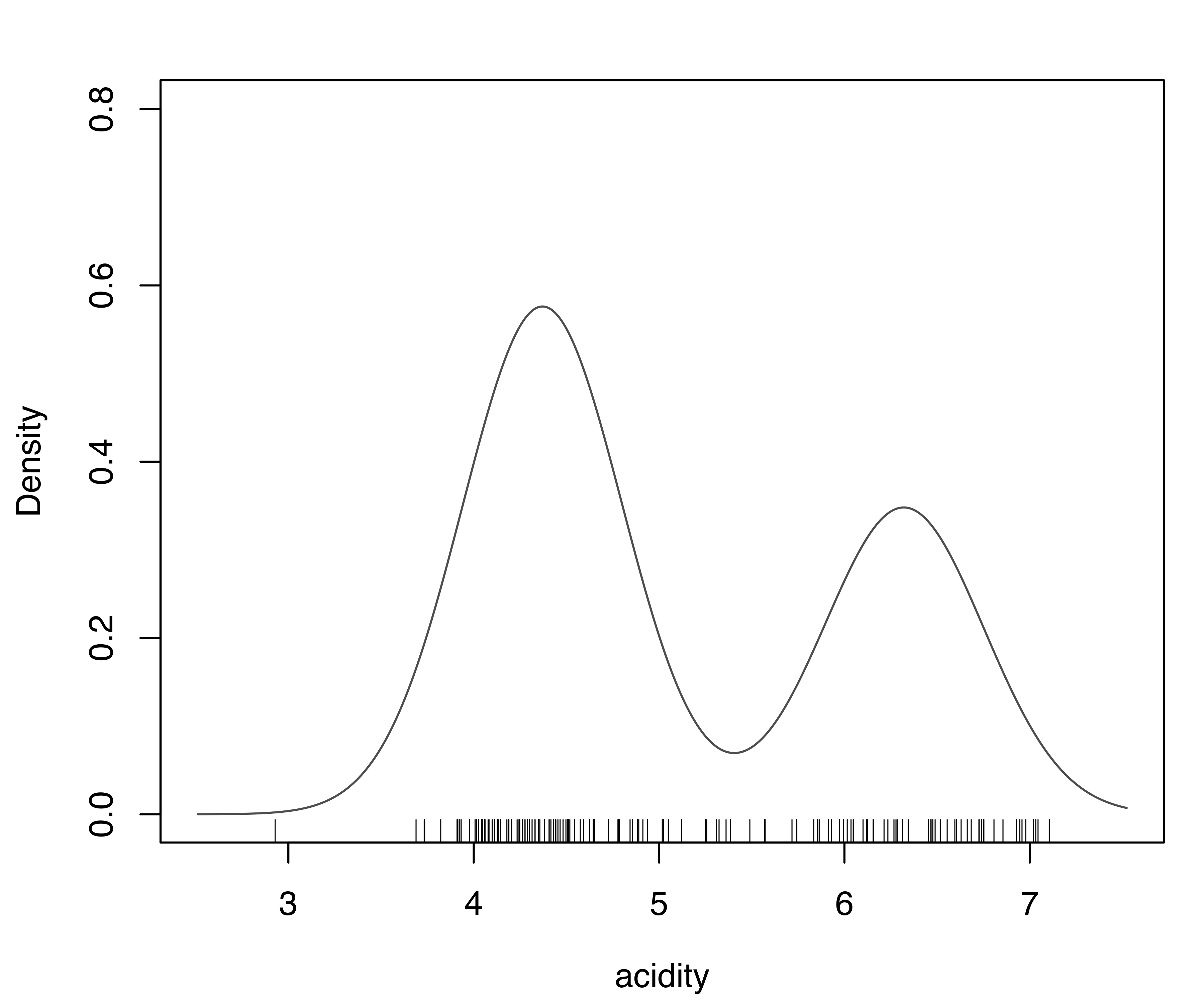
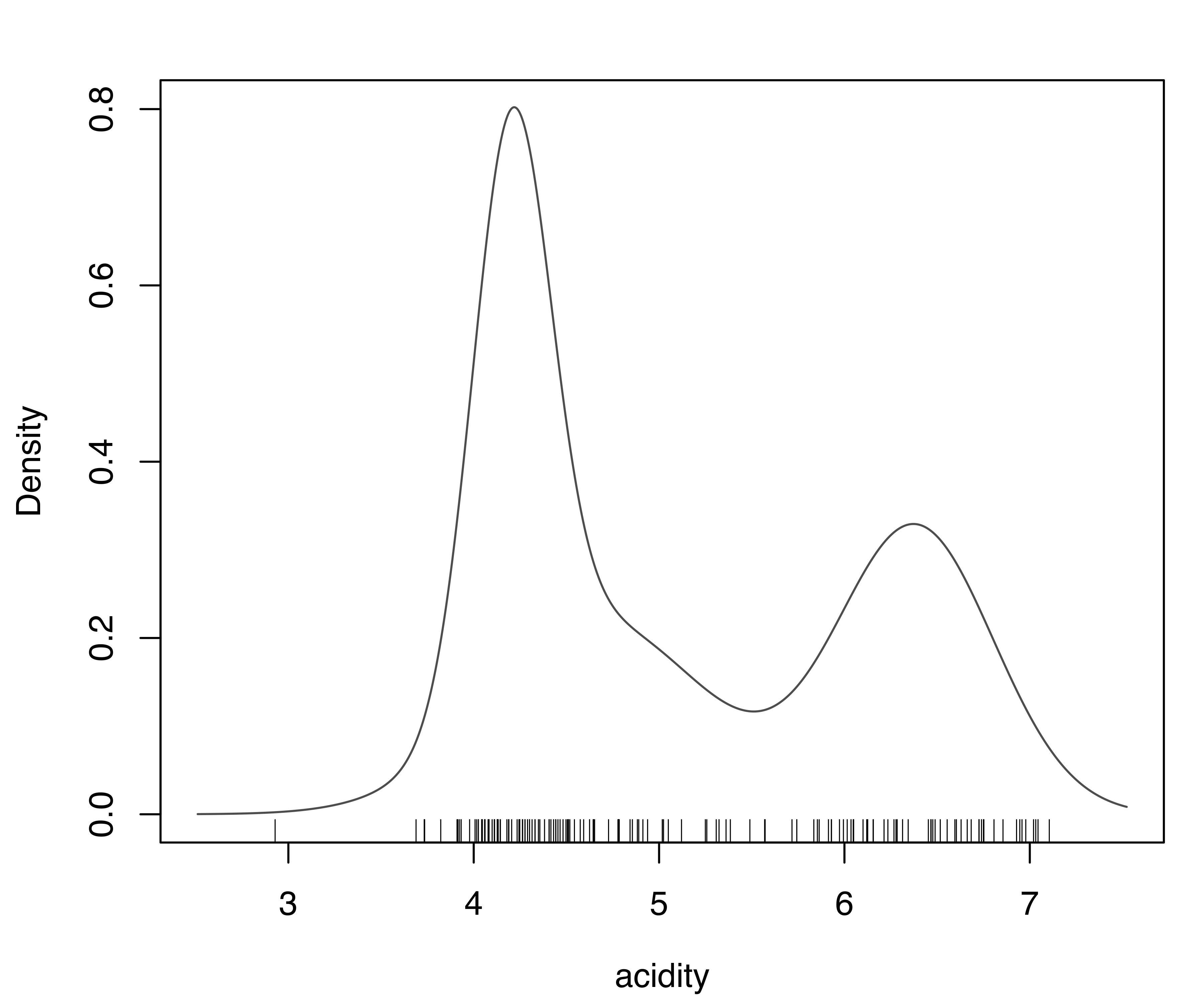
E,2) supported by BIC and (b) the model (V,3) supported by the LRT for the acidity data.
Figure 5.3 shows the plots of the estimated densities. The two models largely agree, with the exception of a somewhat different shape for some lower-range values. In particular, both densities indicate a bimodal distribution.
5.3.1 Diagnostics for Univariate Density Estimation
Two diagnostic plots for density estimation are available for univariate data (for details see Loader 1999, 87–90). The first plot is a graph of the estimated cumulative distribution function (CDF) against the empirical distribution function. The second is a Q-Q plot of the sample quantiles against the quantiles computed from the estimated density. For a GMM, the estimated CDF is just the weighted sum of individual CDFs for each component. It can be obtained in mclust via the function cdfMclust().
Example 5.3 Diagnostic for density estimation of acidity data
Recalling Example 5.2 on acidity data, diagnostic plots for the (E,2) model can be obtained as follows:
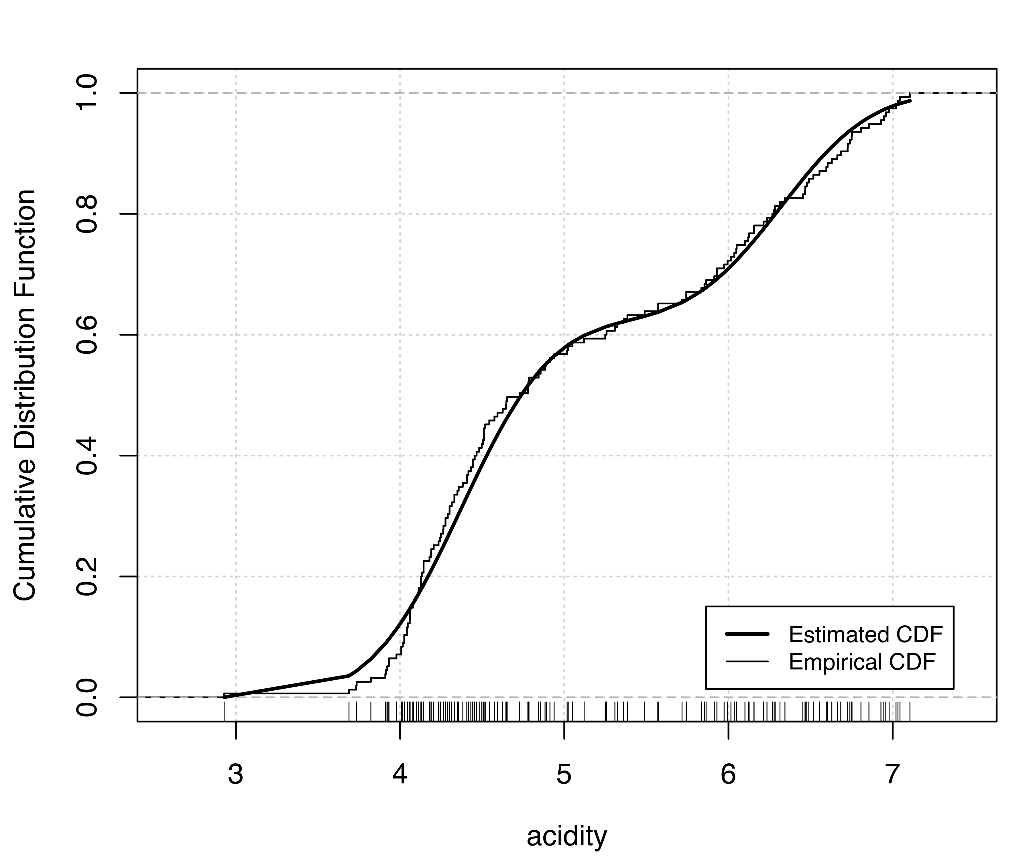
E,2) model estimated for the acidity data: (a) estimated CDF and empirical distribution function, (b) Q-Q plot of sample quantiles vs. quantiles from density estimation.
Similarly, for the model (V,3):
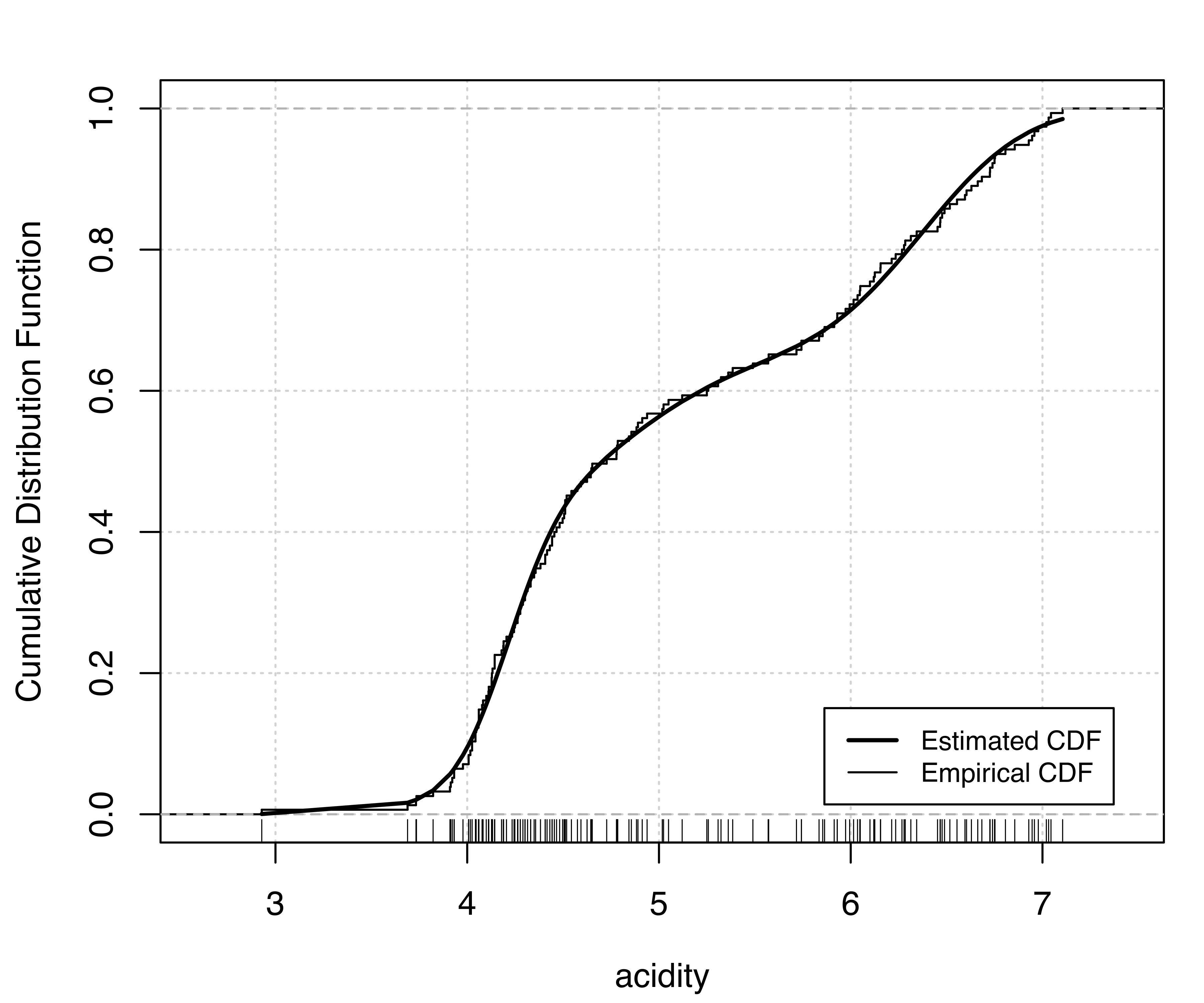

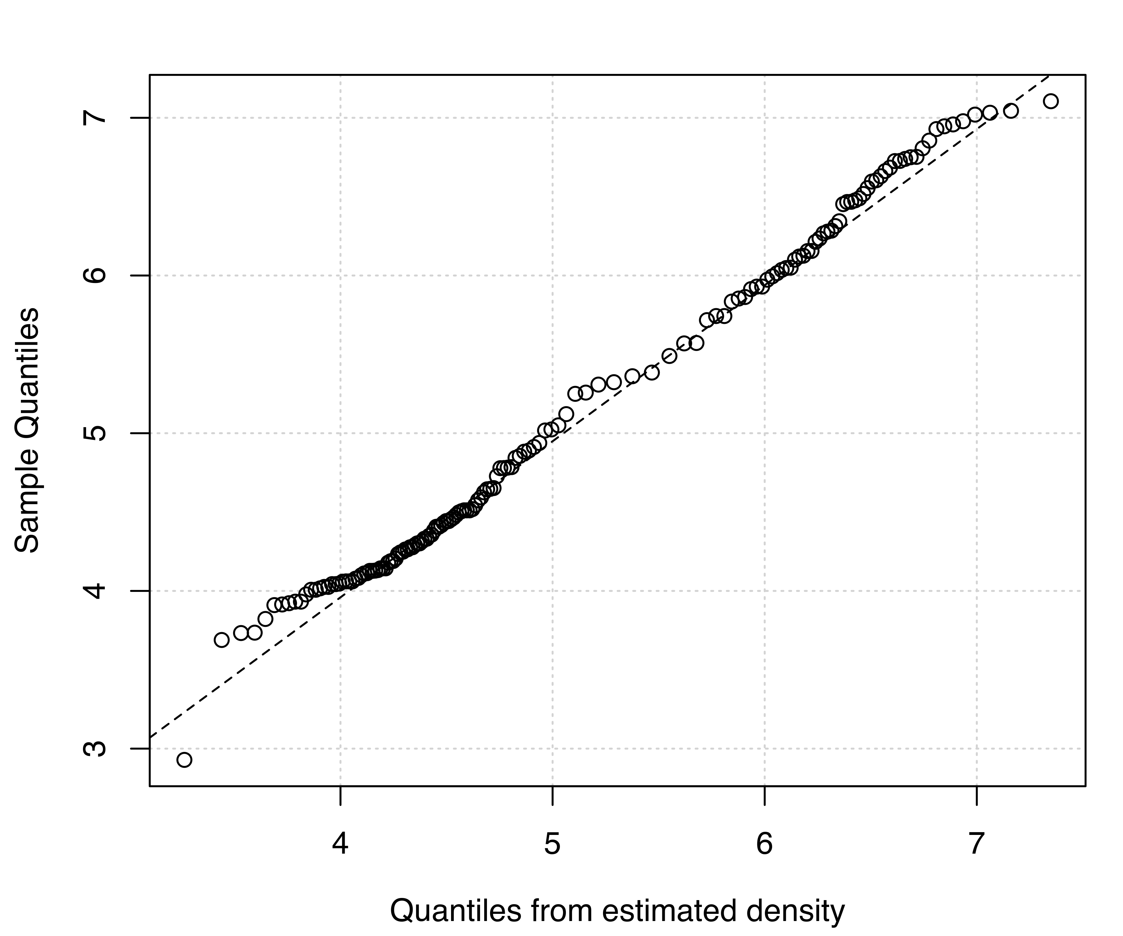
V,3) model estimated for the acidity data: (a) estimated CDF and empirical distribution function, (b) Q-Q plot of sample quantiles vs. quantiles from density estimation.
Figure 5.4 (a) and Figure 5.5 (a) compare the estimated CDFs to the empirical CDF. Figure 5.4 (b) and Figure 5.5 (b) show the corresponding Q-Q plots for the two models. Both types of diagnostics seem to suggest a better fit to the observed data for the more complex model, with perhaps one outlying point corresponding to the smallest value.
5.4 Density Estimation in Higher Dimensions
In principle, density estimation in higher dimensions is straightforward with mclust. The structure imposed by the Gaussian components allows a parsimonious representation of the underlying density, especially when compared to KDE approaches. However, density estimation in high dimensions is problematic in general. Another issue is that visualizing densities beyond three dimensions is difficult. Following the suggestion of (Scott 2009, 217), we should investigate “density estimation in several dimensions rather than in very high dimensions”.
Example 5.4 Density estimation of Old Faithful data
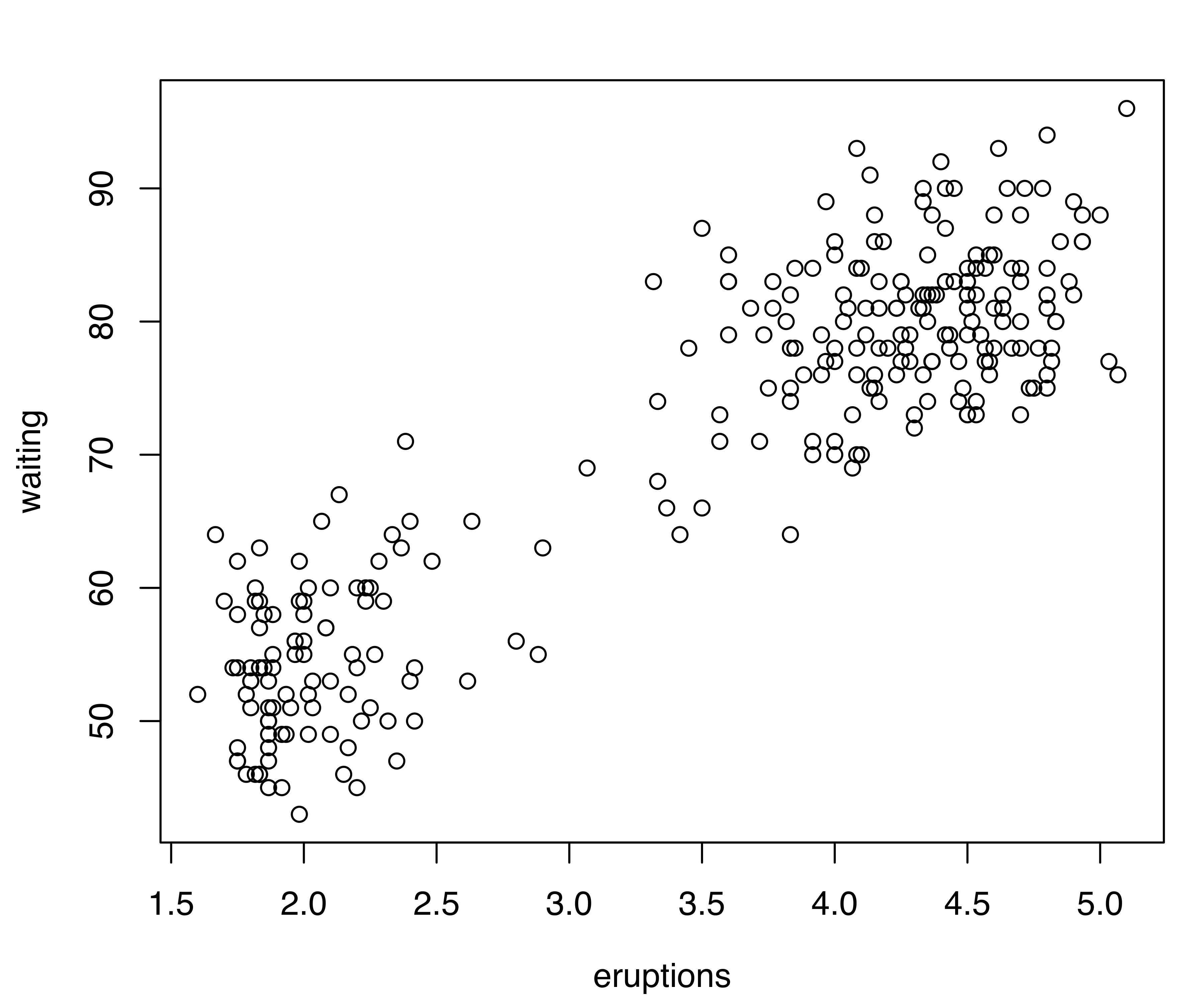
Consider the Old Faithful data described in Example 3.4}. A scatterplot of the data is shown in Figure 5.6 (a). This and the corresponding density estimate can be obtained with the following code:
data("faithful", package = "datasets")
plot(faithful)
dens = densityMclust(faithful)
summary(dens, parameters = TRUE)
## -------------------------------------------------------
## Density estimation via Gaussian finite mixture modeling
## -------------------------------------------------------
##
## Mclust EEE (ellipsoidal, equal volume, shape and orientation) model
## with 3 components:
##
##  log-likelihood   n df     BIC     ICL
##         -1126.3 272 11 -2314.3 -2357.8
##
## Mixing probabilities:
##       1       2       3
## 0.16568 0.35637 0.47795
##
## Means:
##              [,1]    [,2]    [,3]
## eruptions  3.7931  2.0376  4.4632
## waiting   77.5211 54.4912 80.8334
##
## Variances:
## [,,1]
##           eruptions waiting
## eruptions  0.078254  0.4802
## waiting    0.480198 33.7671
## [,,2]
##           eruptions waiting
## eruptions  0.078254  0.4802
## waiting    0.480198 33.7671
## [,,3]
##           eruptions waiting
## eruptions  0.078254  0.4802
## waiting    0.480198 33.7671
Model selection based on the BIC selects a three-component mixture with common covariance matrix (EEE,3). One component is used to model the group of observations having both low duration and low waiting times, whereas two components are needed to approximate the skewed distribution of the observations with larger duration and waiting times.
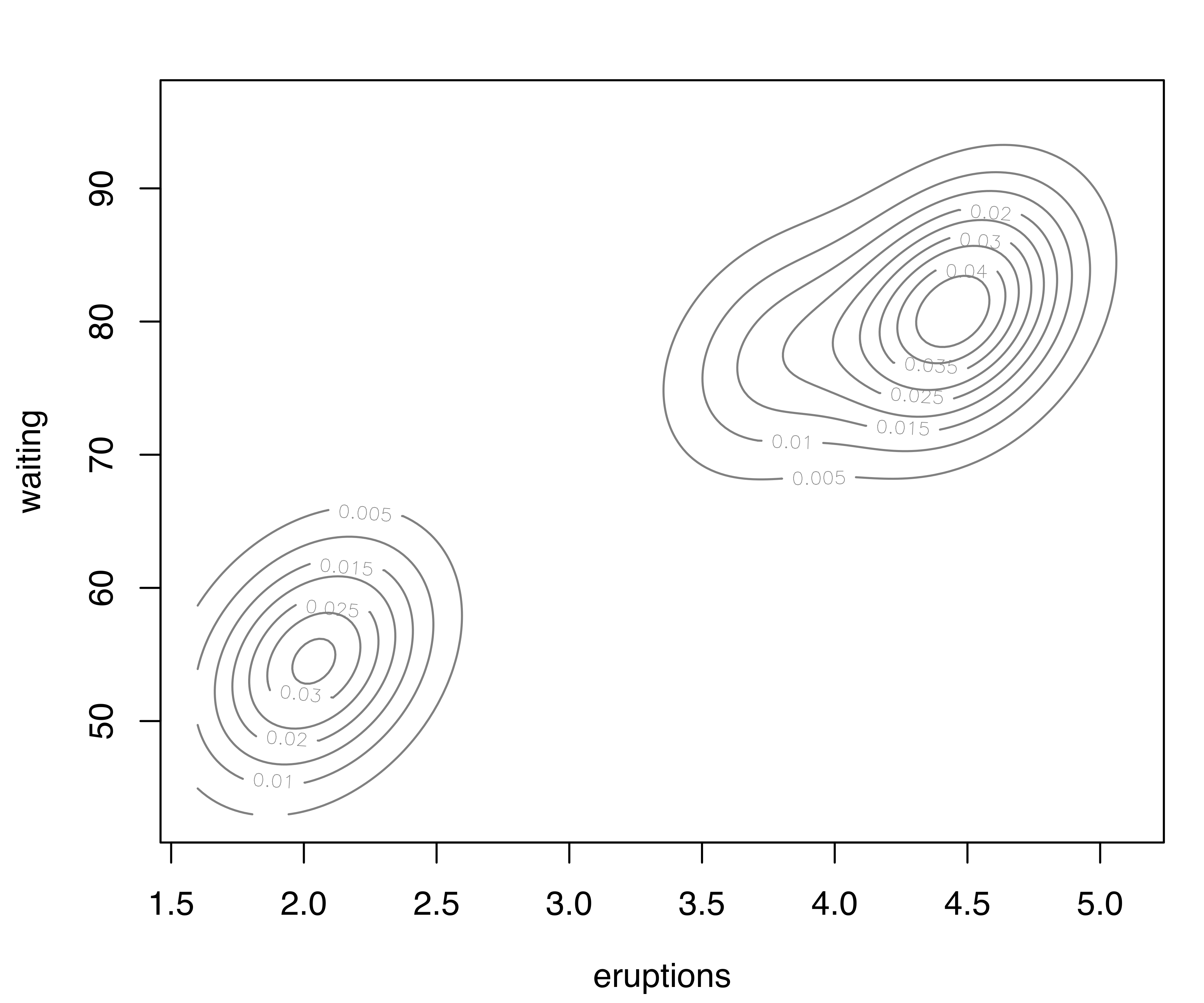
For two-dimensional data, the plot() method for the argument what = "density" is by default a contour plot of the density estimate, as shown in Figure 5.6 (b):
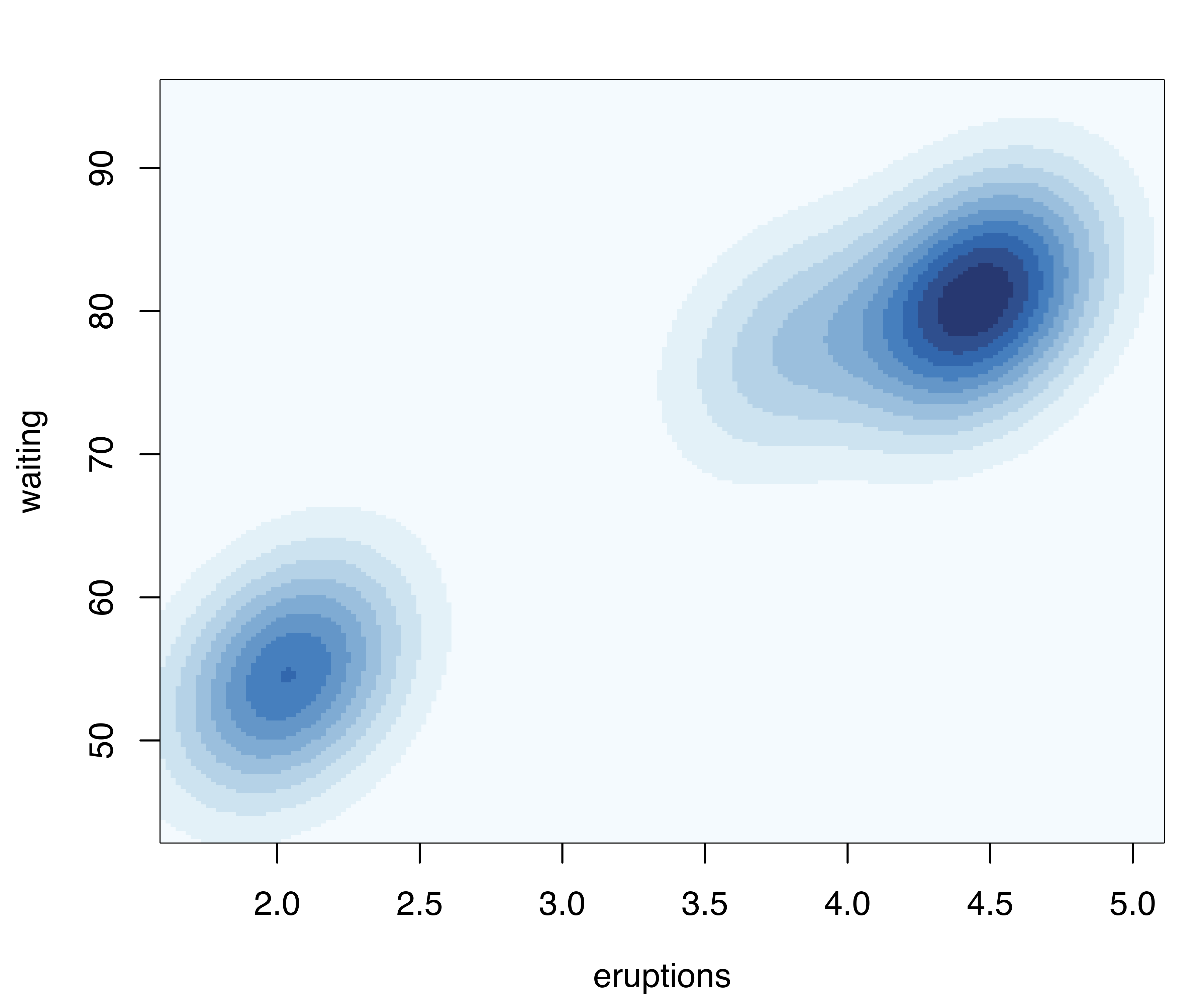
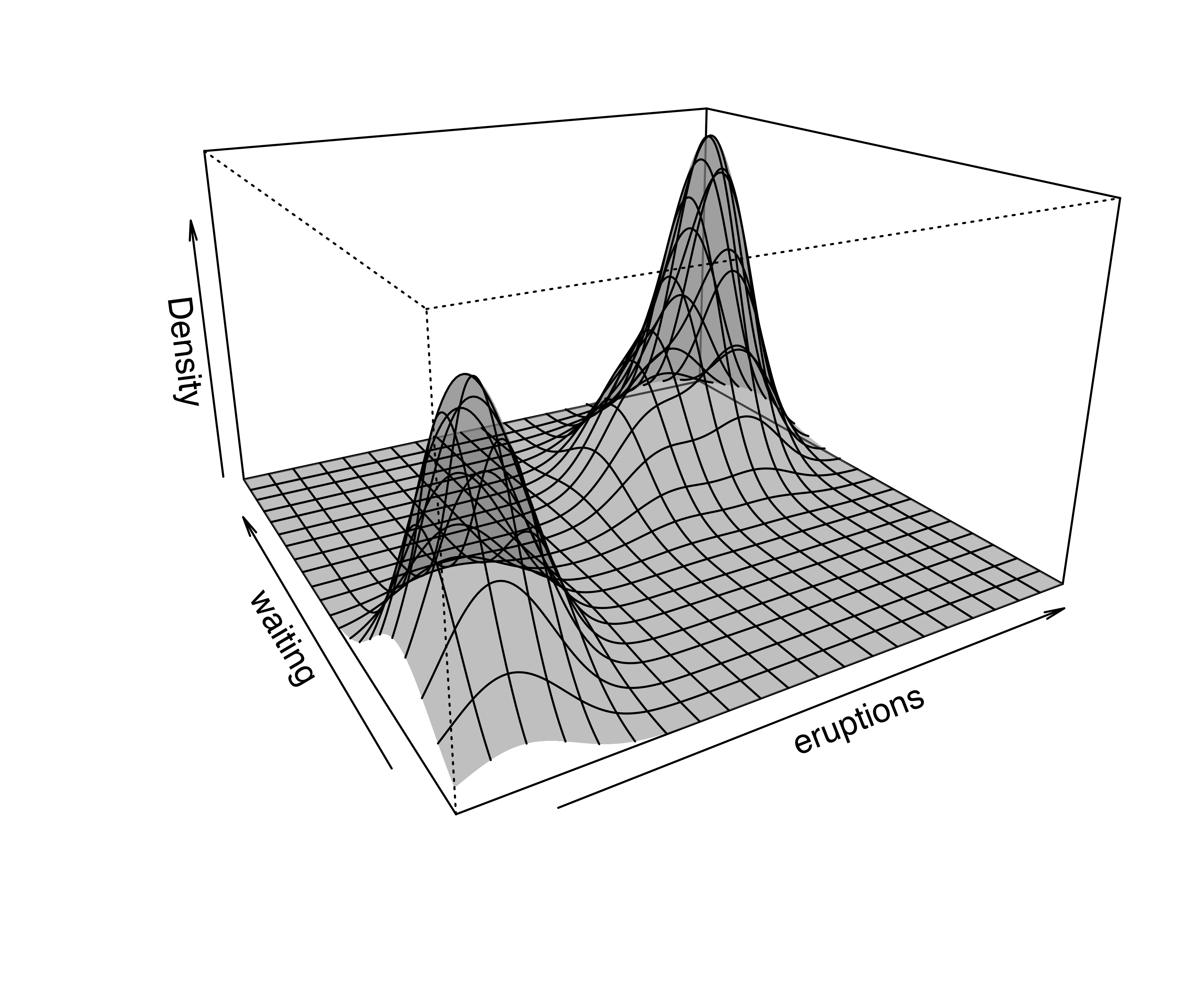
plot(dens, what = "density")A bivariate density estimate may also be plotted using an image plot or a perspective plot (see Figure 5.6 (c) and Figure 5.6 (d)):
In the above code we specified the type of density plot to produce. Several optional arguments for customizing the plots are available; for a complete description see help("plot.densityMclust") and help("surfacePlot"). More details on producing graphical displays with mclust are discussed in Section 6.2 and Section 6.3.
Another useful approach to visualizing multivariate densities involves summarizing a density estimate with (possibly disjoint) regions of the sample space covering a specified probability. These are called Highest Density Regions (HDRs) by Hyndman (1996); for details on the definition and the computational implementation see Section 5.6.
In mclust, HDRs can be easily obtained by specifying type = "hdr" in the plot() function applied to an object returned by a densityMclust() function call:
plot(dens, what = "density", type = "hdr")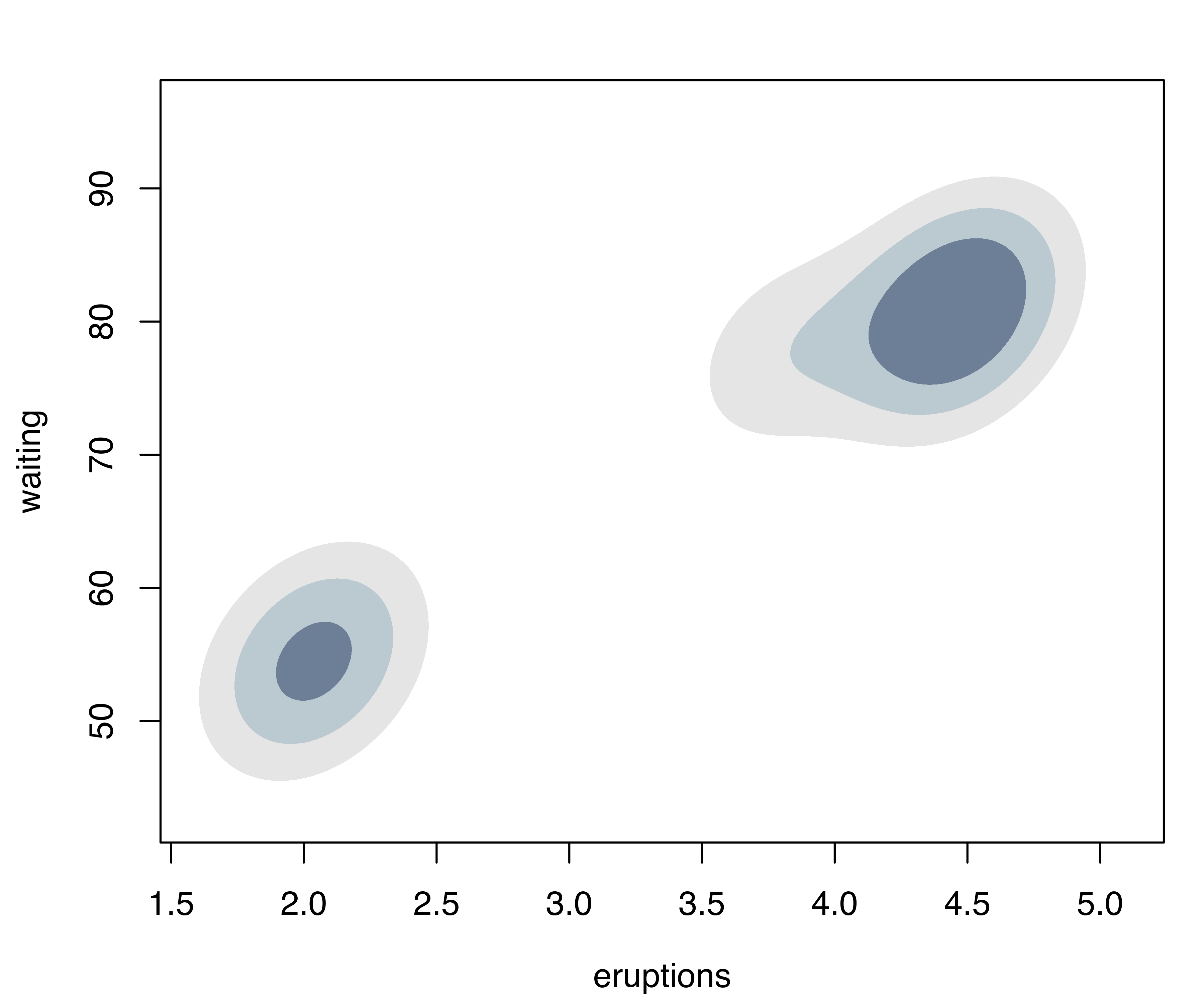
faithful data at probability levels 0.25, 0.5, and 0.75.
For higher dimensional datasets densityMclust() provides graphical displays of density estimates using density contour, image, and perspective plots for pairs of variables arranged in a matrix.
Example 5.5 Density estimation on principal components of the aircraft data
Consider the dataset aircraft, available in the sm package (A. Bowman et al. 2022) for R, giving measurements on six physical characteristics of twentieth-century aircraft. Following the analysis of A. W. Bowman and Azzalini (1997, sec. 1.3), we consider the principal components computed from the data on the log scale for the time period 1956–1984:
data("aircraft", package = "sm")
X = log(subset(aircraft, subset = (Period == 3), select = 3:8))
PCA = prcomp(X, scale = TRUE)
summary(PCA)
## Importance of components:
##                          PC1   PC2    PC3     PC4     PC5     PC6
## Standard deviation     2.085 1.064 0.6790 0.16892 0.15239 0.08771
## Proportion of Variance 0.725 0.189 0.0769 0.00476 0.00387 0.00128
## Cumulative Proportion  0.725 0.913 0.9901 0.99485 0.99872 1.00000
PCA$rotation       # loadings
##             PC1       PC2      PC3        PC4       PC5       PC6
## Power  -0.45612  0.262445  0.11357 -0.2267760 -0.565774 -0.581940
## Span   -0.37433 -0.540127  0.32461 -0.5305967  0.417040 -0.085530
## Length -0.46737 -0.088898  0.21657  0.7885789  0.260671 -0.192237
## Weight -0.47409  0.036498  0.17017 -0.0121226 -0.365831  0.781647
## Speed  -0.29394  0.731054 -0.15713 -0.2121675  0.551014  0.076387
## Range  -0.34963 -0.309371 -0.88384  0.0045952 -0.024057 -0.016386
Z = PCA$x[, 1:3]   # PCA projection
Consider the fit of a GMM on the first three principal components (PCs), which explain 99% of total variability. The BIC criterion indicates a number of candidate models with almost the same support from the data.
BIC = mclustBIC(Z)
summary(BIC, k = 5)
## Best BIC values:
##            VEE,5        VVE,4      VEI,6     VVE,3      VEE,4
## BIC      -1958.7 -1958.752723 -1961.8724 -1962.876 -1965.7162
## BIC diff     0.0    -0.014737    -3.1344    -4.138    -6.9782
We fit the simpler three-component model with varying volume and shape (VVE), and plot the estimated density (see Figure 5.8).
densAircraft = densityMclust(Z, G = 3, modelNames = "VVE", plot = FALSE)
plot(densAircraft, what = "density", type = "hdr",
     data = Z, points.cex = 0.5)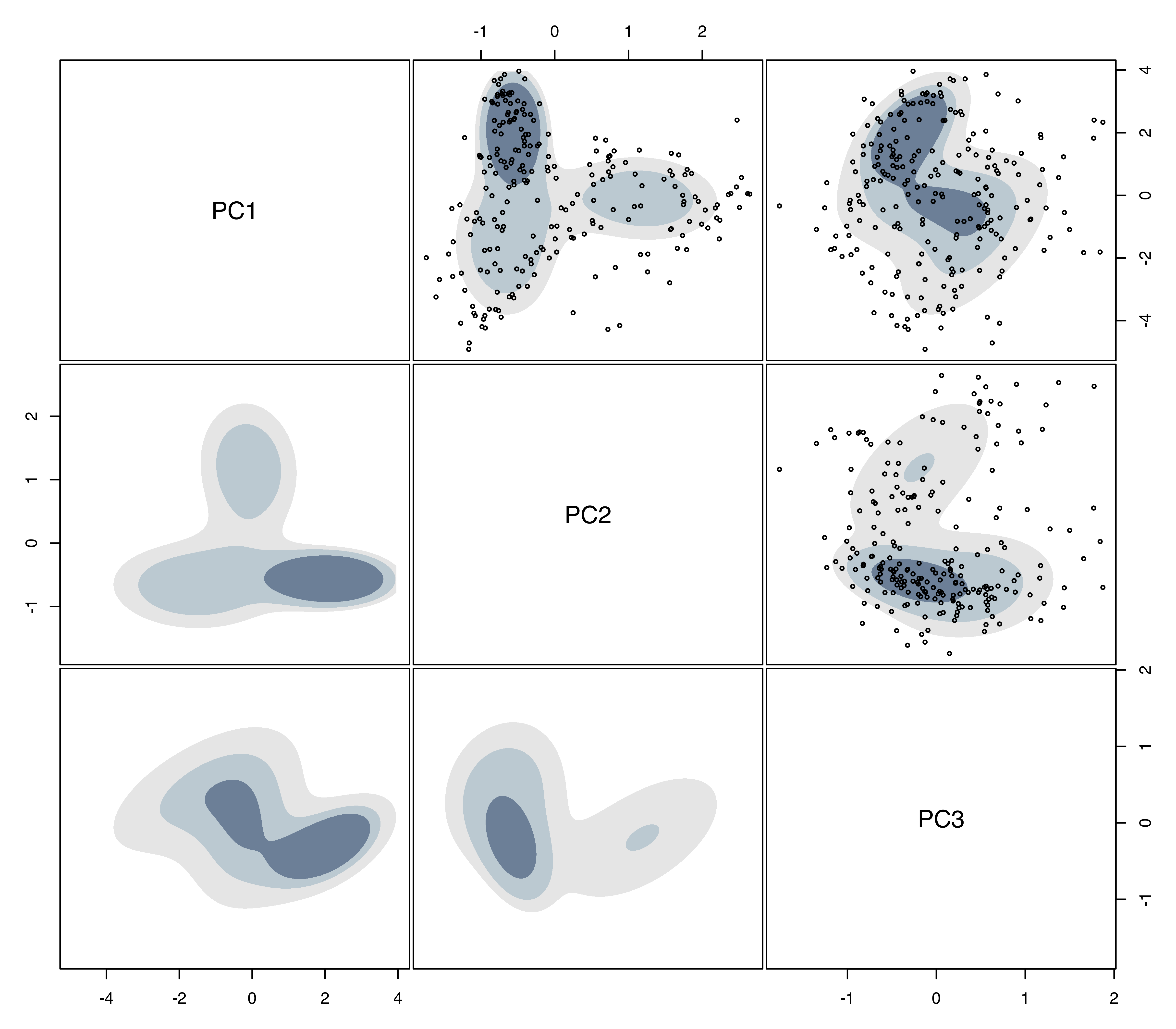
aircraft data with bivariate highest density regions at probability levels 0.25, 0.5, and 0.75.
The default probability levels \(0.25\), \(0.5\), and \(0.75\) are used in these plots (for details see Section 5.6). The plots are arranged in a symmetric matrix, where each off-diagonal panel shows the bivariate marginal density estimate. Data points have been also added to the upper-diagonal panels by providing the matrix of principal components to the optional argument data. The presence of several modes is clearly evident from this figure.
5.5 Density Estimation for Bounded Data
Finite mixtures of Gaussian distributions provide a flexible model for density estimation when the continuous variables under investigation have no boundaries. However, in practical applications variables may be partially bounded (taking non-negative values) or completely bounded (taking values in the unit interval). In this case, the standard Gaussian finite mixture model assigns non-zero densities to any possible value, even to those outside the ranges where the variables are defined, hence resulting in potentially severe bias.
A transformation-based approach for Gaussian mixture modeling in the case of bounded variables has been recently proposed (Scrucca 2019). The basic idea is to carry out density estimation not on the original data \(\boldsymbol{x}\) with bounded support \(\mathcal{S}_{\mathcal{X}} \subset \Real^d\), but on the transformed data \(\boldsymbol{y}= t(\boldsymbol{x}; \boldsymbol{\lambda})\) having unbounded support \(\mathcal{S}_{\mathcal{Y}}\). A range-power transformation is used for \(t(\cdot ; \boldsymbol{\lambda})\). This is a monotonic transformation which depends on parameters \(\boldsymbol{\lambda}\) and maps \(\mathcal{S}_{\mathcal{X}}\) to \(\mathcal{S}_{\mathcal{Y}}\). The range part of the transformation differs depending on whether a variable has only a lower bound or has both a lower and an upper bound, while the power part of the transformation involves the well-known Box-Cox transformation (Box and Cox 1964). Once the density on the transformed scale is estimated, the density for the original data can be obtained by a change of variables using the Jacobian of the transformation. Both the transformation parameters and the parameters of the Gaussian mixture are jointly estimated by the EM algorithm. For more details see Scrucca (2019).
The methodology briefly outlined above is implemented in the R package mclustAddons (Scrucca 2022):
Example 5.6 Density estimation of suicide data
The dataset gives the lengths (in days) of 86 spells of psychiatric treatment undergone by control patients in a suicide risk study (Silverman 1998). Since the variable can only take positive values, in the following we contrast the density estimated ignoring this fact with the estimate obtained using the approach outlined above.
The following code estimates the density using the function densityMclust() with its default settings:
data("suicide", package = "mclustAddons")
dens = densityMclust(suicide)
rug(suicide)            # add data points at the bottom of the graph
abline(v = 0, lty = 3)  # draw a vertical line at the natural boundary
The resulting density is shown in Figure 5.9 (a). This is clearly unsatisfactory because it assigns nonzero density to negative values and exhibits a bimodal distribution, the latter being an artifact due to failure to account for the non-negativity.
The function densityMclustBounded() can be used for improved density estimation by specifying the lower bound of the variable:
bdens = densityMclustBounded(suicide, lbound = 0)
summary(bdens, parameters = TRUE)
## ── Density estimation for bounded data via GMMs ───────────
##
## Boundaries: suicide
##       lower       0
##       upper     Inf
##
## Model E (univariate, equal variance) model with 1 component
## on the transformation scale:
##
##  log-likelihood  n df   BIC   ICL
##         -497.82 86  3 -1009 -1009
##
##                             suicide
## Range-power transformation: 0.19293
##
## Mixing probabilities:
## 1
## 1
##
## Means:
##      1
## 6.7001
##
## Variances:
##      1
## 7.7883
plot(bdens, what = "density")
rug(suicide)            # add data points at the bottom of the graph
abline(v = 0, lty = 3)  # draw a vertical line at the natural boundary
The estimated parameter of the range-power transformation is equal to \(0.19\), and on the transformed scale the optimal GMM is a model with a single mixture component. The corresponding density estimate on the original scale of the variable is shown in Figure 5.9 (b). As the plot shows, accounting for the natural boundary of the variable better represents the underlying density of the data.
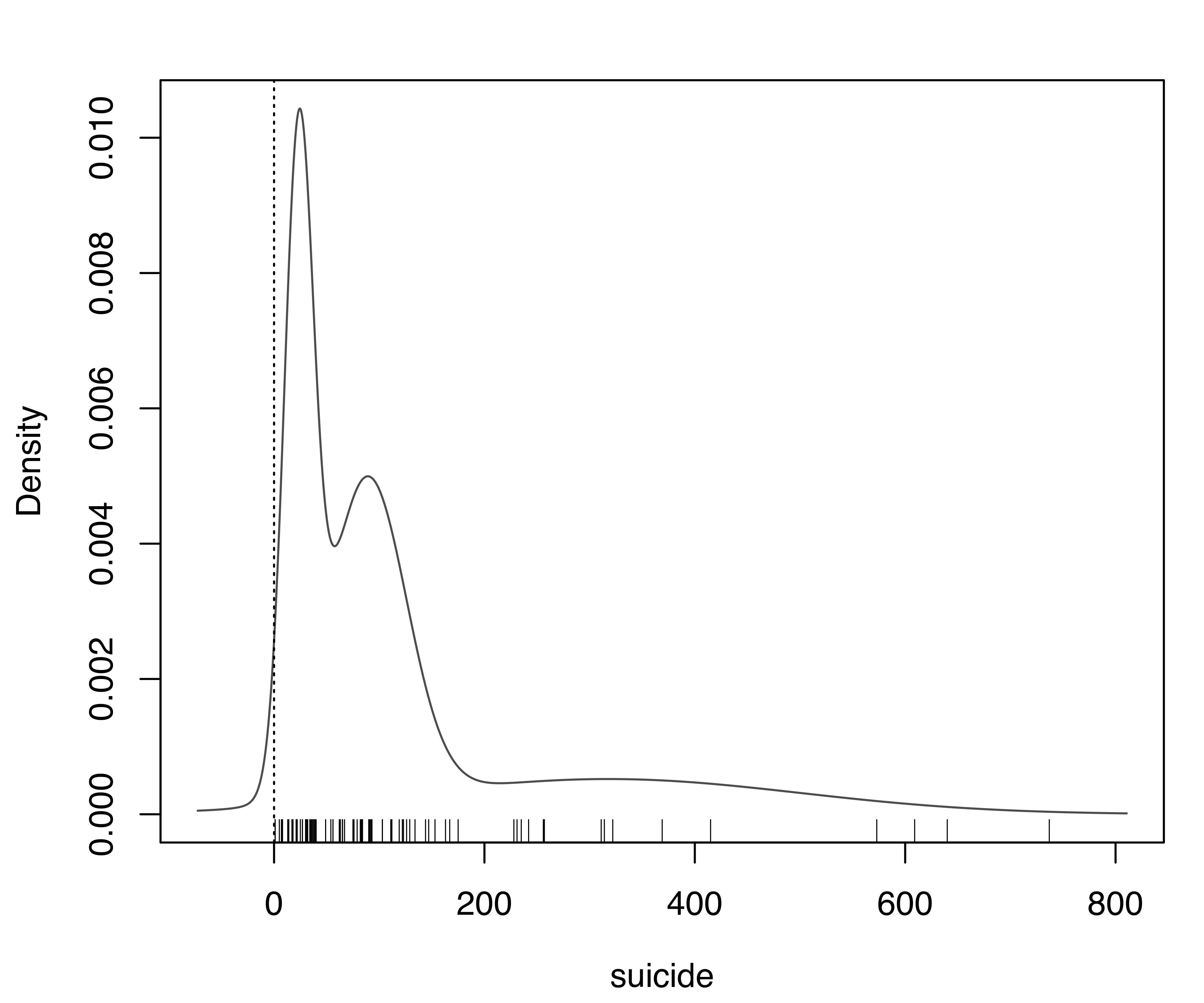
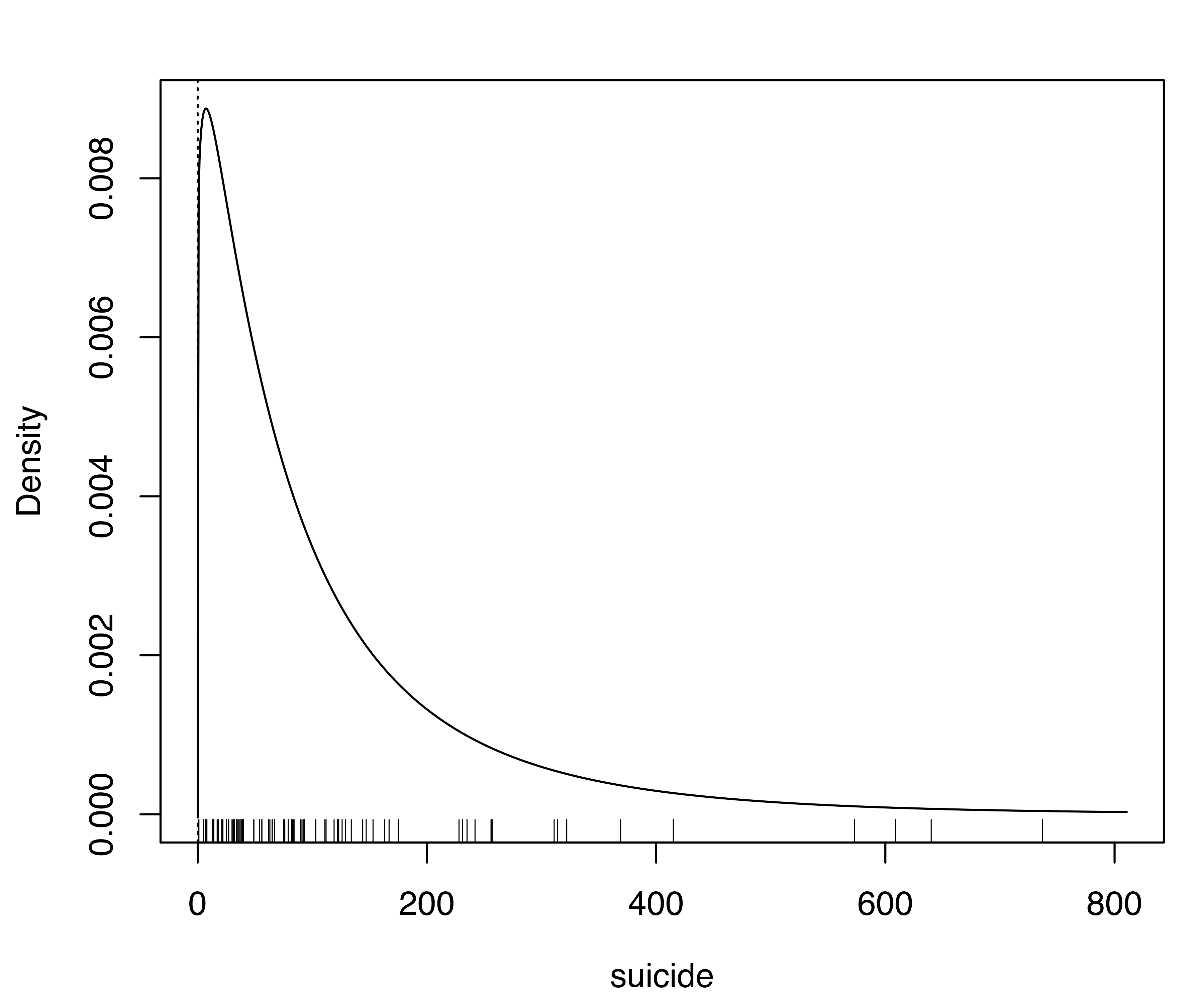
suicide data. Panel (a) shows the default estimate which ignores the lower boundary of the variable, while panel (b) shows the density estimated accounting for the natural boundary of the variable.
Example 5.7 Density estimation of racial data
This dataset provides the proportion of white student enrollment in 56 school districts in Nassau County (Long Island, New York, USA), for the 1992–1993 school year (Simonoff 1996, sec. 3.2). Because each observation is a proportion, the density estimate for this data should not fall outside the \([0,1]\) range.
The following code reads the data, performs density estimation by specifying both the lower and upper bounds of the variable under study, and plots the data and the estimated density:
data("racial", package = "mclustAddons")
bdens = densityMclustBounded(racial$PropWhite, lbound = 0, ubound = 1)
plot(bdens, what = "density",
     lwd = 2, col = "dodgerblue2",
     data = racial$PropWhite, breaks = 15,
     xlab = "Proportion of white students enrolled in schools")
rug(racial$PropWhite)        # add data points at the bottom of the graph
abline(v = c(0, 1), lty = 3)  # draw a vertical line at the natural boundary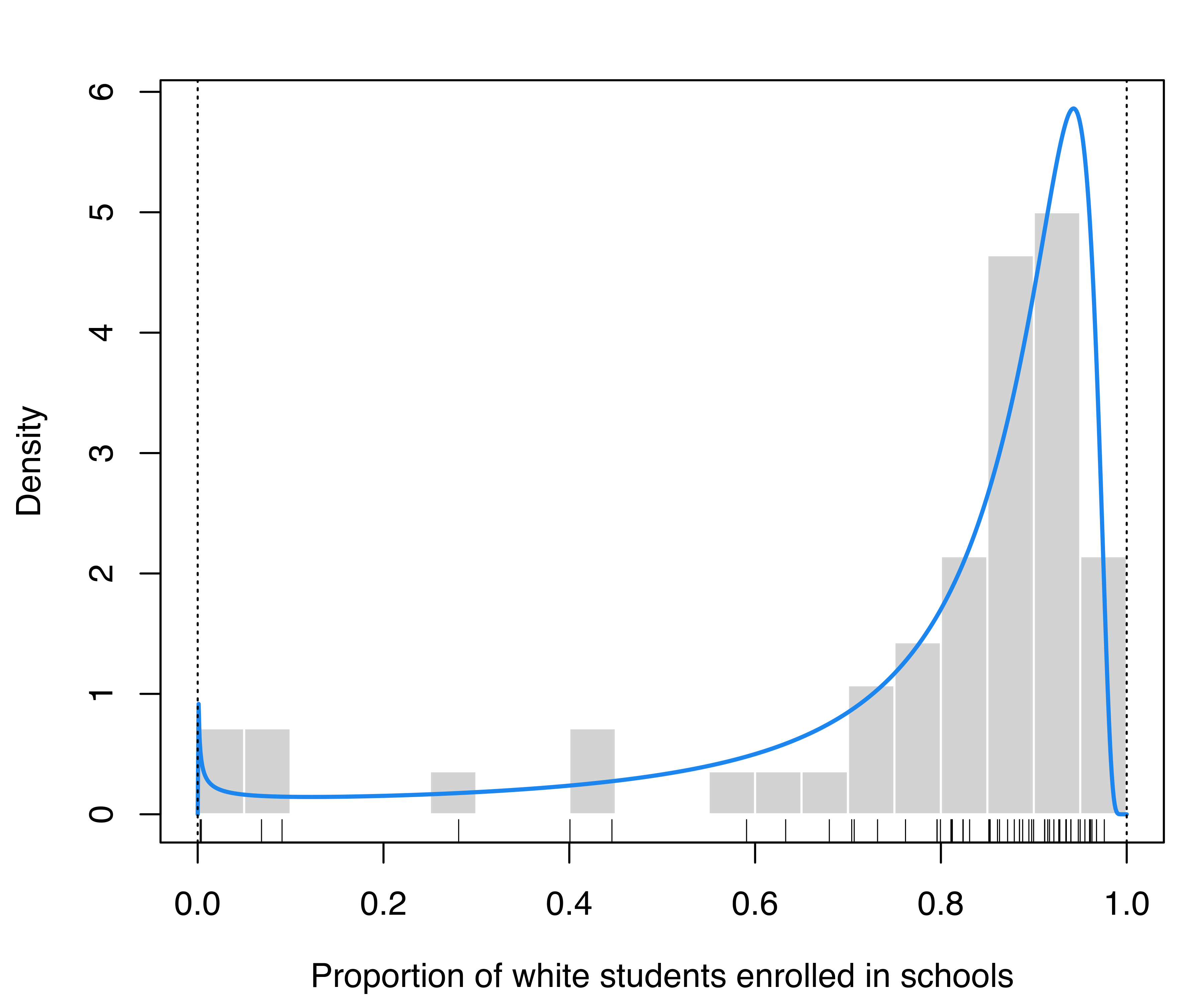
racial data obtained by taking into account the natural boundary of the proportion.
Figure 5.10 displays the estimated density, showing that the majority of the schools have at least 70% of white students, but there is also a small peak near the lower boundary containing schools with almost 0% of white students.
5.6 Highest Density Regions
Density curves are a very effective and useful way to show the distribution of values in a dataset. For two-dimensional data, perspective and contour plots represent a standard way to visualize densities (see for instance Figure 5.6). An alternative method is discussed by Hyndman (1996), who proposed the use of Highest Density Regions (HDRs) for summarizing probability distributions. These are defined as the (possibly disjoint) regions of the sample space covering a specified probability level.
Let \(f(x)\) be the density function of a random variable \(X\); then the \(100(1-\alpha)\%\) HDR is the subset \(R(f_\alpha)\) of the sample space of \(X\) such that \[ R(f_\alpha) = \{x : f(x) \ge f_\alpha \}, \] where \(f_\alpha\) is the largest value such that \(\Pr( X \in R(f_\alpha)) \ge 1-\alpha\).
For estimating \(R(f_\alpha)\), Hyndman (1996) proposed considering the \((1-\alpha)\)-quantile of the density function evaluated at the observed data points. The accuracy of this method depends on the sample size, so for small to moderate sample sizes the degree of accuracy can be improved by enlarging the set of observations with additional simulated data points.
For example, consider the density of a univariate two-component Gaussian mixture defined with the following code and shown in Figure 5.11:
f = function(x)
  0.7*dnorm(x, mean = 0, sd = 1) + 0.3*dnorm(x, mean = 4, sd = 1)
curve(f, from = -4, to = 8)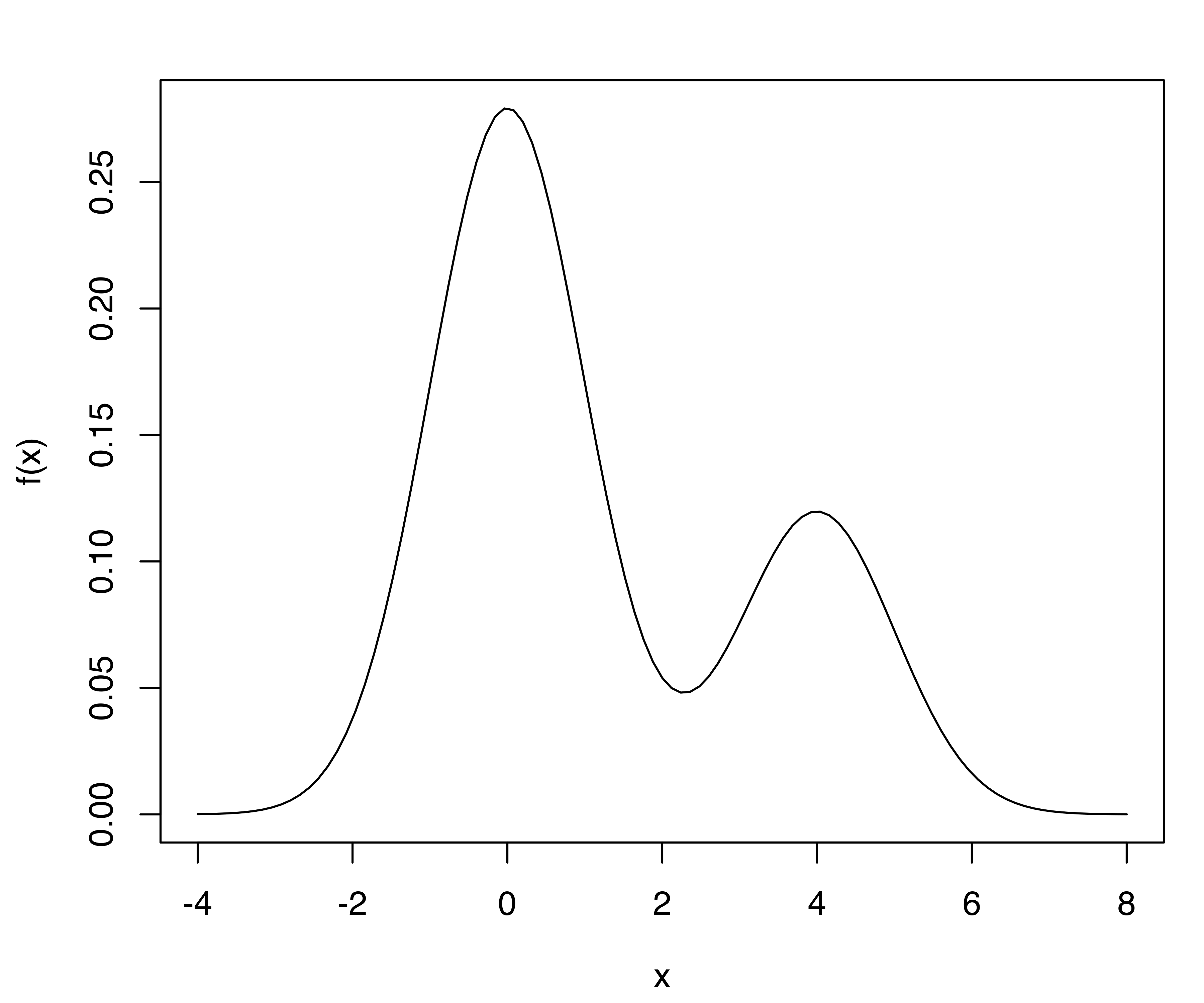
A simulated dataset drawn from this mixture can be obtained as follows:
The first column returned by sim() contains the (randomly generated) classification and is therefore omitted. For details of the procedure, see Section 7.4.
The highest density regions corresponding to specified probability levels can be computed using the function hdrlevels(), and then plotted as follows:
(hdr = hdrlevels(f(x), prob))
##      25%      50%      75%      95%
## 0.250682 0.158753 0.096956 0.048063
for (j in seq(prob))
{
  curve(f, from = -4, to = 8)
  mtext(side = 3, paste0(prob[j]*100, "% HDR"), adj = 0)
  abline(h = hdr[j], lty = 2)
  rug(x, col = "lightgrey")
  rug(x[f(x) >= hdr[j]])
}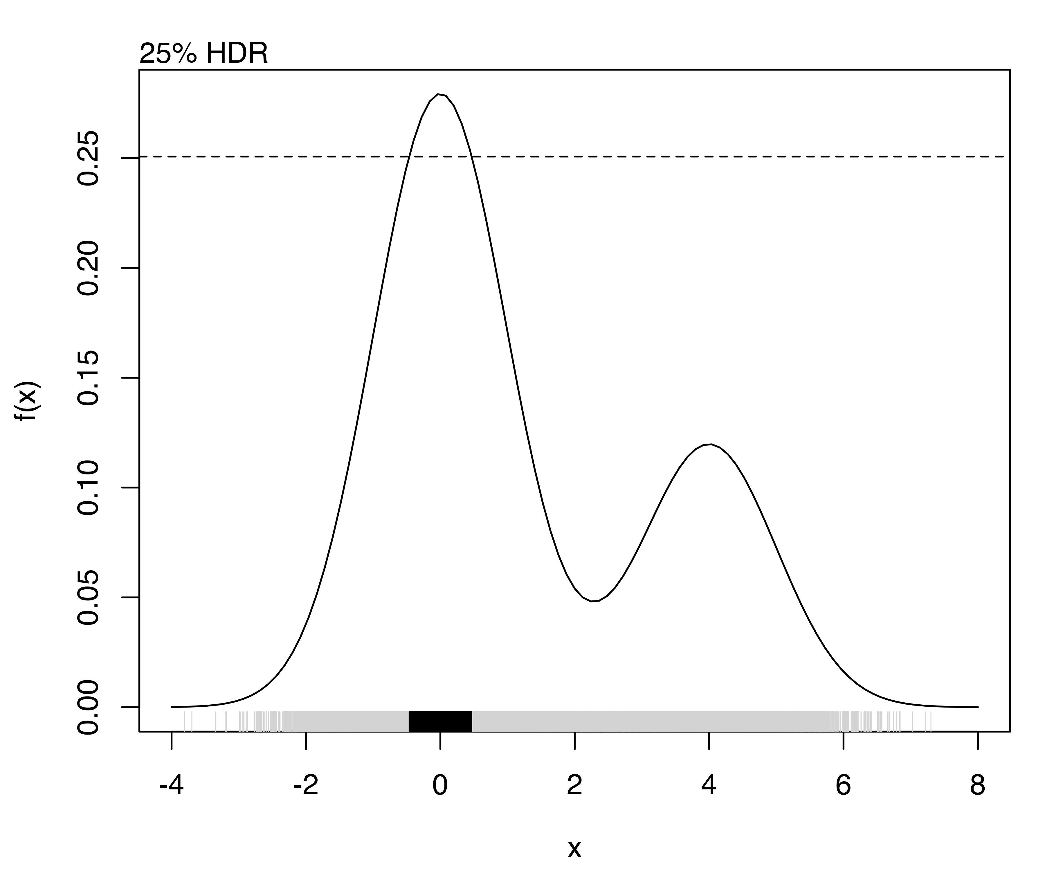
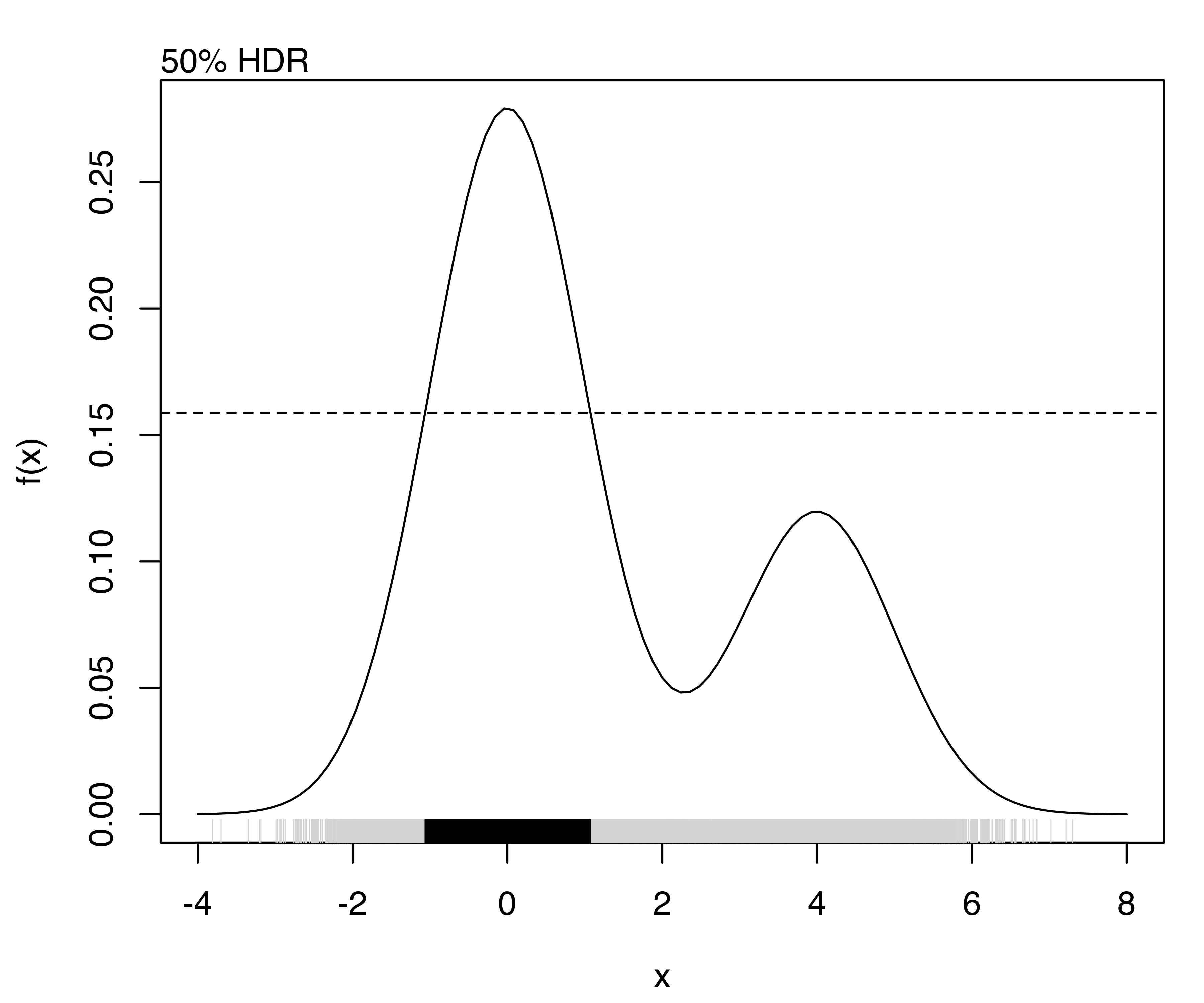
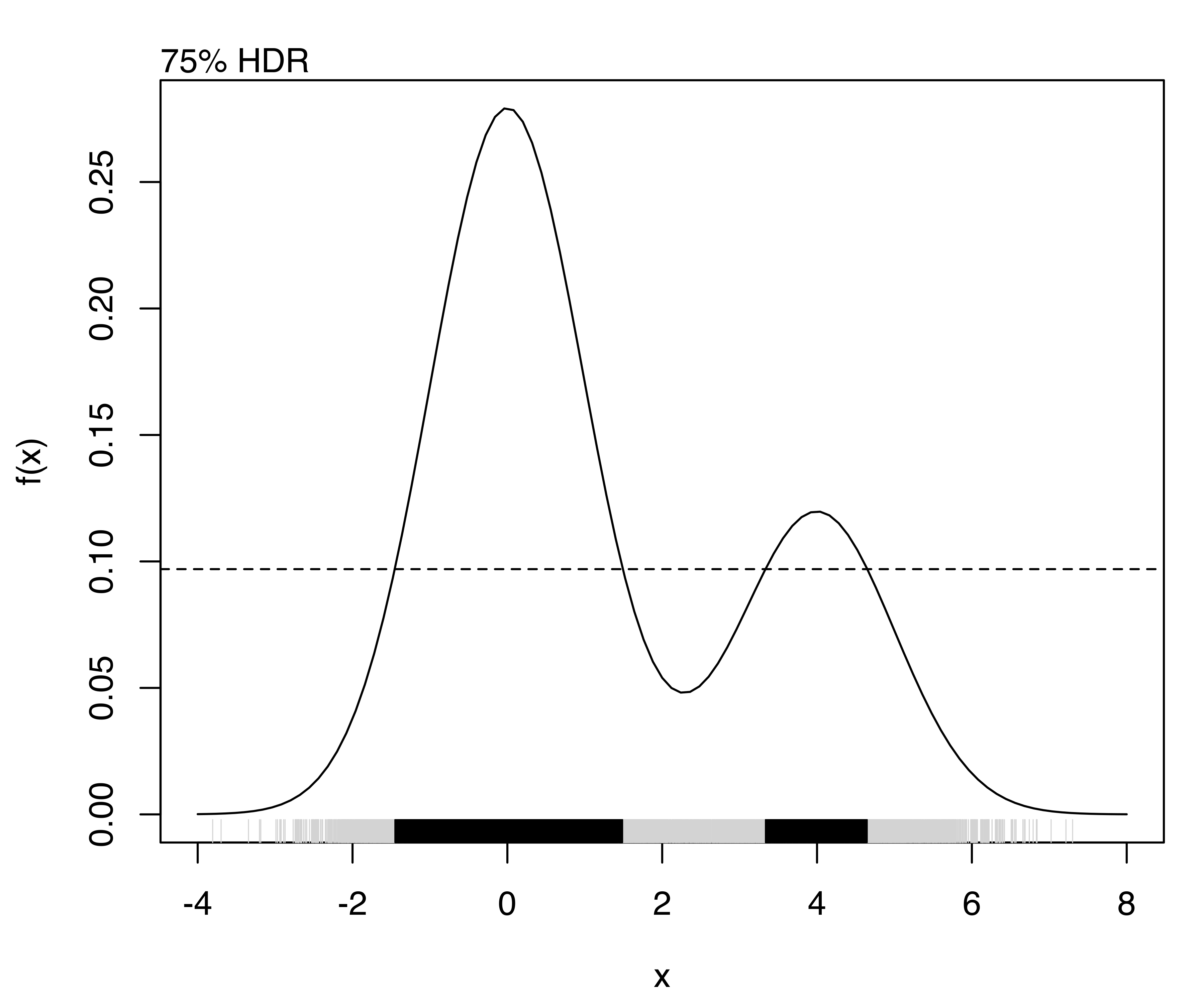
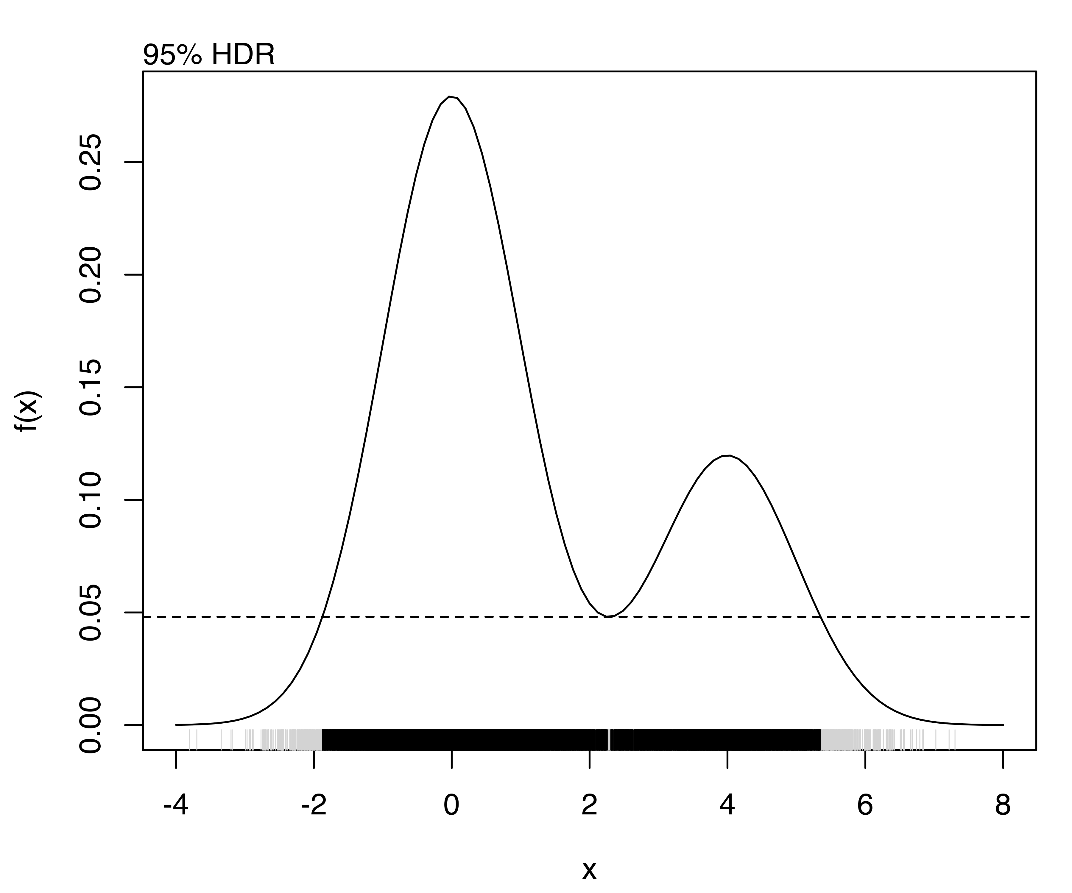
The resulting plots are shown in Figure 5.12.
In general the true density function is unknown, so that an estimate must be used, but the procedure remains essentially unchanged. For instance, we may estimate the density with mclust and then obtain the HDR levels as follows:
dens = densityMclust(x, plot = FALSE)
hdrlevels(predict(dens, x), prob)
##      25%      50%      75%      95%
## 0.251234 0.159436 0.096781 0.048798