4 Mixture-Based Classification
\[ \DeclareMathOperator{\Real}{\mathbb{R}} \DeclareMathOperator{\Proj}{\text{P}} \DeclareMathOperator{\Exp}{\text{E}} \DeclareMathOperator{\Var}{\text{Var}} \DeclareMathOperator{\var}{\text{var}} \DeclareMathOperator{\sd}{\text{sd}} \DeclareMathOperator{\cov}{\text{cov}} \DeclareMathOperator{\cor}{\text{cor}} \DeclareMathOperator{\range}{\text{range}} \DeclareMathOperator{\rank}{\text{rank}} \DeclareMathOperator{\ind}{\perp\hspace*{-1.1ex}\perp} \DeclareMathOperator{\CE}{\text{CE}} \DeclareMathOperator{\BS}{\text{BS}} \DeclareMathOperator{\ECM}{\text{ECM}} \DeclareMathOperator{\BSS}{\text{BSS}} \DeclareMathOperator{\WSS}{\text{WSS}} \DeclareMathOperator{\TSS}{\text{TSS}} \DeclareMathOperator{\BIC}{\text{BIC}} \DeclareMathOperator{\ICL}{\text{ICL}} \DeclareMathOperator{\CV}{\text{CV}} \DeclareMathOperator{\diag}{\text{diag}} \DeclareMathOperator{\se}{\text{se}} \DeclareMathOperator{\Cov}{\text{Cov}} \DeclareMathOperator{\boot}{\text{boot}} \DeclareMathOperator{\LRTS}{\text{LRTS}} \DeclareMathOperator{\Model}{\mathcal{M}} \DeclareMathOperator*{\argmin}{arg\min} \DeclareMathOperator*{\argmax}{arg\max} \DeclareMathOperator{\vech}{vech} \DeclareMathOperator{\tr}{tr} \]
Classification is an instance of supervised learning, where the class of each observation is known. Unlike in the unsupervised case, the main objective here is to build a classifier for classifying future observations. This chapter describes probabilistic classification following a mixture-based approach. It describes various Gaussian mixture models for supervised learning. The implementation available in mclust is presented using several data analysis examples. Different ways of assessing classifier performance are also discussed. The problem of unequal costs of misclassification and the classification with unbalanced classes is presented, followed by solutions implemented in mclust. The chapter concludes with an introduction to the semi-supervised classification problems, in which only some of the training data have known labels.
4.1 Classification as Supervised Learning
Chapter 3 discussed methods for clustering, an instance of unsupervised learning. There the main goal was to identify the presence of groups of homogeneous observations based on the measurements available for a set of variables or features. This chapter deals with the supervised learning problem, where the classification of each observation is known. In this case, the main objective is to build a classifier (or decision rule) for classifying future observations from the available data (Bishop 2006; T. Hastie, Tibshirani, and Friedman 2009; Alpaydin 2014). This task is also known by various other names, such as statistical pattern recognition or discriminant analysis (G. McLachlan 2004).
In the probabilistic approach to classification, a statistical model is estimated to predict the class \(C_k\) for \(k=1, \dots, K\) of a given observation with feature vector \(\boldsymbol{x}\). This model provides a posterior class probability \(\Pr(C_k|\boldsymbol{x})\) for each class, which can then be used to determine the class membership for new observations. Some modeling methods directly estimate posterior probabilities by constructing, or learning, a discriminant function \(\eta_k(\boldsymbol{x}) = \Pr(C_k|\boldsymbol{x})\) that maps the features \(\boldsymbol{x}\) directly onto a class \(C_k\). These are called discriminative models, of which a popular instance is the logistic regression model for binary-class problems.
Other approaches try to explicitly or implicitly model the distribution of features as well as classes, and then obtain the posterior probabilities using Bayes’ theorem. Thus, by learning the class-conditional densities \(f(\boldsymbol{x}|C_k)\) and the prior class probabilities \(\Pr(C_k)\) for each class \(C_k\) (\(k=1, \dots, K\)), the posterior class probabilities are given by% can be found as \[ \Pr(C_k|\boldsymbol{x}) = \frac{f(\boldsymbol{x}|C_k) \Pr(C_k)}{\displaystyle\sum_{g=1}^K f(\boldsymbol{x}|C_g) \Pr(C_g)} . \] Methods that follow this approach, such as those based on finite mixture modeling, are called generative models.
Typically, classification models are estimated using the information from a training set, meaning a dataset used for learning or fitting the model in order to obtain parameter estimates. The same dataset, if used also for model tuning such as hyperparameter estimation or feature selection and for evaluating the classifier, tends to produce an optimistic assessment of performance. This phenomenon is called overfitting, meaning that there is a risk of fitting a model that too closely corresponds to a particular set of data, and therefore may fail to fit additional data or predict future observations well. For these reasons, it is advisable to perform model tuning using a validation set, a dataset designed for this purpose and usually set aside from the original dataset. An alternative is to repeatedly split into a training set and a validation set using resampling approaches, such as cross-validation, to be discussed in Section 4.4.3. Another subset of the original dataset is also set aside in advance as a test set for the final evaluation of the classifier.
4.2 Gaussian Mixture Models for Classification
Consider a training dataset \(\mathcal{D}_\text{train}= \{(\boldsymbol{x}_1, y_1), \dots, (\boldsymbol{x}_n, y_n)\}\) for which both the feature vectors \(\boldsymbol{x}_i\) and the true classes \(y_i \in \{C_1, \dots, C_K\}\) are known. Each observation has an associated class label \(C_k\).
Mixture-based classification models typically assume that the density within each class follows a Gaussian mixture distribution: \[ f(\boldsymbol{x}|C_k) = \sum_{g=1}^{G_k} \pi_{g,k} \phi(\boldsymbol{x}; \boldsymbol{\mu}_{g,k}, \boldsymbol{\Sigma}_{g,k}), \tag{4.1}\] where \(G_k\) is the number of components within class \(k\), \(\pi_{g,k}\) are the mixing probabilities for class \(k\) (\(\pi_{g,k} > 0\) and \(\sum_{g=1}^{G_k}\pi_{g,k}=1\)), and \(\boldsymbol{\mu}_{g,k}\) and \(\boldsymbol{\Sigma}_{g,k}\) are, respectively, the mean vectors and the covariance matrices for component \(g\) within class \(k\).
Trevor Hastie and Tibshirani (1996) proposed the Mixture Discriminant Analysis (MDA) model where it is assumed that the covariance matrix is the same for all classes but is otherwise unconstrained (\(\boldsymbol{\Sigma}_{gk} = \boldsymbol{\Sigma}\) for all \(g=1,\dots,G_k\) and \(k=1,\dots,K\) in Equation 4.1). Moreover, the number of mixture components is the same for each class and assumed known.
Bensmail and Celeux (1996) proposed the Eigenvalue Decomposition Discriminant Analysis (EDDA) model which assumes that the density for each class can be described by a single Gaussian component (\(G_k=1\) for all \(k\) in Equation 4.1), with the class covariance structure factorized as \[ \boldsymbol{\Sigma}_{k} = \lambda_k\boldsymbol{U}_k\boldsymbol{\Delta}_k\boldsymbol{U}{}^{\!\top}_k. \]
As for GMM clustering, several classification models can be obtained from the above decomposition. If each component has the same covariance matrix (\(\boldsymbol{\Sigma}_{k} = \lambda\boldsymbol{U}\boldsymbol{\Delta}\boldsymbol{U}{}^{\!\top}\) — model EEE in Table 2.1), then EDDA is equivalent to the classical Linear Discriminant Analysis (LDA) model. If the component covariance matrices are unconstrained and vary between components (\(\boldsymbol{\Sigma}_{k} = \lambda_k\boldsymbol{U}_k\boldsymbol{\Delta}_k\boldsymbol{U}{}^{\!\top}_k\) — model VVV in Table 2.1), then EDDA is equivalent to the Quadratic Discriminant Analysis (QDA) model. Finally, by assuming conditional independence of features within each class (models with coordinate axes orientation, denoted by **I in Table 2.1), the Naïve-Bayes models are obtained.
The most general model from Equation 4.1 is the MclustDA model proposed by Fraley and Raftery (2002), which uses a finite mixture of Gaussian distributions within each class, in which the number of components and covariance matrix (parameterized by the eigen-decomposition described in Section 2.2.1) may differ among classes.
4.2.1 Prediction
Let \(\tau_k\) be the class prior probability that an observation \(\boldsymbol{x}\) comes from class \(C_k\) (\(k=1,\dots,K\)). By Bayes’ theorem we can compute the posterior probability that an observation \(\boldsymbol{x}\) belongs to class \(C_k\) as \[ \Pr(C_k | \boldsymbol{x}) = \frac{\tau_k f(\boldsymbol{x}| C_k)}{\displaystyle\sum_{j=1}^K \tau_{j} f(\boldsymbol{x}| C_{j})}, \tag{4.2}\] where \(f(\boldsymbol{x}|C_k)\) is the probability density function in Equation 4.1 specific to class \(C_k\). As discussed earlier, this density depends on the assumed model for within-class distributions.
Thus an observation \(\boldsymbol{x}\) can be classified according to the maximum a posteriori (MAP) rule to the class which has the highest posterior probability: \[ y = \{ C_{\widehat{k}} \} \qquad\text{where}\quad \widehat{k} = \argmax_{k} \Pr(C_k | \boldsymbol{x}) \propto \tau_k f(\boldsymbol{x}| C_k), \tag{4.3}\] where the right-hand side follows by noting that the denominator in Equation 4.2 is just a constant of normalization. This rule minimizes the expected misclassification rate and is known as the Bayes classifier.
4.2.2 Estimation
The parameters of the model in Equation 4.1 can be estimated from the training dataset by maximum likelihood. In particular, for the EDDA model the parameters can be obtained with a single M-step from the EM algorithm for Gaussian mixtures described in Section 2.2.2, with \(z_{ik}\) set to \(1\) if observation \(i\) belongs to class \(k\) and \(0\) otherwise. For the general MclustDA model, as well as for MDA, a Gaussian mixture model can be estimated separately for each class using the EM algorithm, and parameters cannot be constrained across classes.
For the class prior probabilities, if the training data have been obtained by random sampling from the underlying population, the mixing proportions \(\tau_k\) can be simply estimated by the sample proportions \(n_k/n\), where \(n_k\) denotes the number of observations known to belong to class \(k\) and \(n = \sum_{k=1}^K n_k\) is the number of observations in the training set. However, there are instances in which different values have to be assigned to the prior probabilities for the classes.
This includes cases where the cost of misclassification may differ depending on the affected classes, and cases where classes have very different numbers of members. These issues are further discussed in Section 4.6 and Section 4.5, respectively.
4.3 Classification in mclust
The main function available in mclust for classification tasks is MclustDA(), which requires a data frame or a matrix for the training data (data) and the corresponding vector of class labels (class). The type of mixture model to be fitted is specified by the argument modelType, a string that can take the values "MclustDA" (default) or "EDDA".
Example 4.1 Classification of Wisconsin diagnostic breast cancer data
Consider a dataset of measurements for 569 patients on 30 features of the cell nuclei obtained from a digitized image of a fine needle aspirate (FNA) of a breast mass [Street, Wolberg, and Mangasarian (1993); Mangasarian:etal:1995], available as one of several contributions to the “Breast Cancer Wisconsin (Diagnostic) Data Set” of the UCI Machine Learning Repository (Dua and Graff 2017). For each patient, the mass was diagnosed as either malignant or benign. This data can be obtained in mclust via the data command under the name wdbc. Following Mangasarian, Street, and Wolberg (1995) and Fraley and Raftery (2002),we consider only three attributes in the following analysis: extreme area, extreme smoothness, and mean texture.
We randomly assign approximately two-thirds of the observations to the training set, and the remaining ones to the test set, as follows:
set.seed(123)
train = sample(1:nrow(X), size = round(nrow(X)*2/3), replace = FALSE)
X_train = X[train, ]
Class_train = Class[train]
tab = table(Class_train)
cbind(Counts = tab, "%" = prop.table(tab)*100)
##   Counts      %
## B    251 66.227
## M    128 33.773
X_test = X[-train, ]
Class_test = Class[-train]
tab = table(Class_test)
cbind(Counts = tab, "%" = prop.table(tab)*100)
##   Counts      %
## B    106 55.789
## M     84 44.211
The distribution of the features with training data points marked according to cancer diagnosis is shown in Figure 4.1:
clp = clPairs(X_train, Class_train, lower.panel = NULL)
clPairsLegend(0.1, 0.3, col = clp$col, pch = clp$pch,
              class = ifelse(clp$class == "B", "Benign", "Malign"),
              title = "Breast cancer diagnosis:")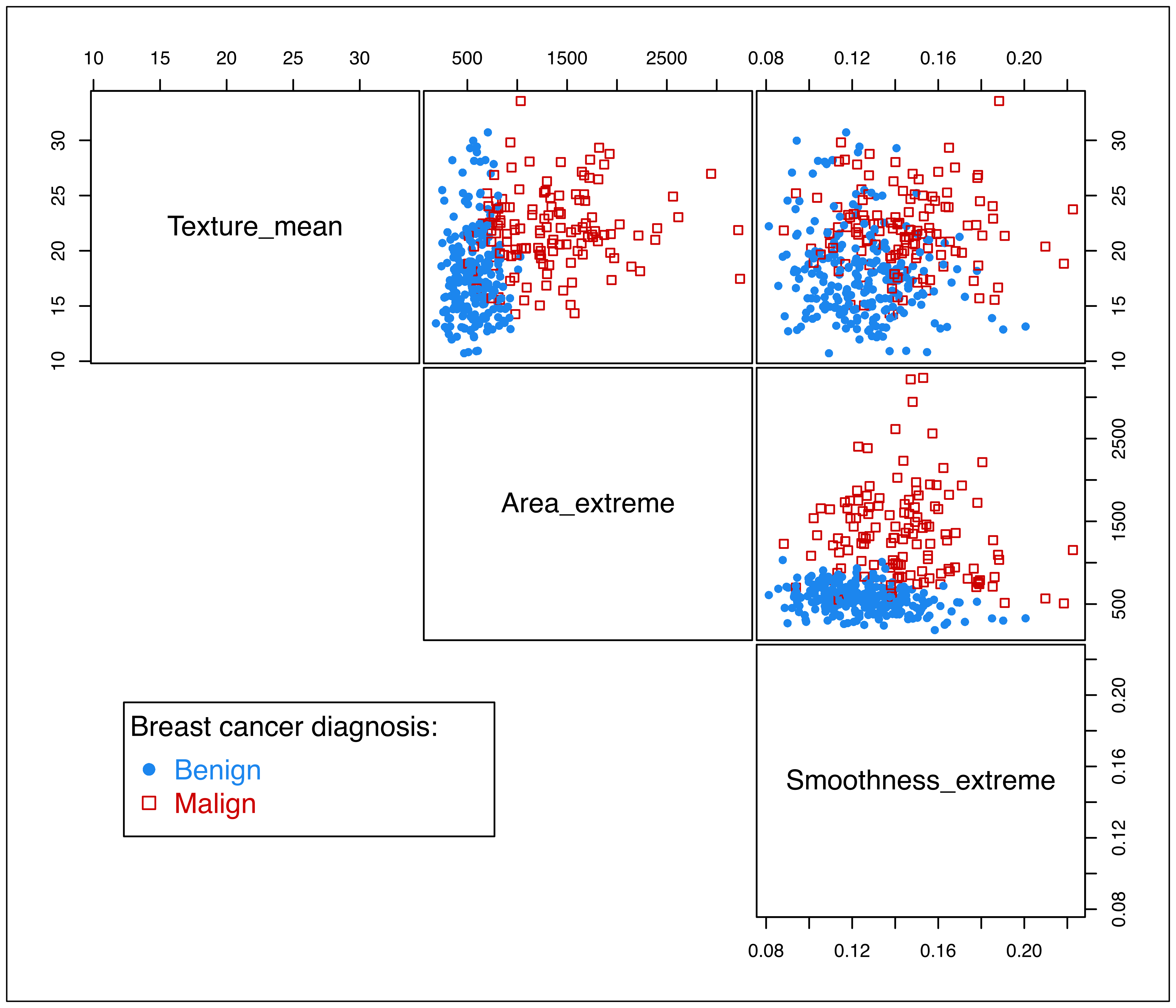
The function MclustDA() provides fitting capabilities for the EDDA model by specifying the optional argument modelType = "EDDA". The corresponding function call is as follows:
mod1 = MclustDA(X_train, Class_train, modelType = "EDDA")
summary(mod1)
## ------------------------------------------------
## Gaussian finite mixture model for classification
## ------------------------------------------------
##
## EDDA model summary:
##
##  log-likelihood   n df     BIC
##         -2934.1 379 13 -5945.4
##
## Classes   n     % Model G
##       B 251 66.23   VVI 1
##       M 128 33.77   VVI 1
##
## Training confusion matrix:
##      Predicted
## Class   B   M
##     B 249   2
##     M  17 111
## Classification error = 0.0501
## Brier score          = 0.0374
The estimated EDDA mixture model with the largest BIC is the VVI model, in which each group is described by a single Gaussian component with varying volume and shape, and orientation aligned with the coordinate axes. As mentioned earlier, this model is a member of the Naïve-Bayes family. By default, the summary() function also returns the confusion matrix obtained by cross-tabulation of the input and predicted classes, followed by two measures of accuracy to be discussed in Section 4.4.
Estimated parameters can be shown with the summary() function by setting the optional argument parameters as follows:
summary(mod1, parameters = TRUE)
## ------------------------------------------------
## Gaussian finite mixture model for classification
## ------------------------------------------------
##
## EDDA model summary:
##
##  log-likelihood   n df     BIC
##         -2934.1 379 13 -5945.4
##
## Classes   n     % Model G
##       B 251 66.23   VVI 1
##       M 128 33.77   VVI 1
##
## Class prior probabilities:
##       B       M
## 0.66227 0.33773
##
## Class = B
##
## Means:
##                         [,1]
## Texture_mean        17.95530
## Area_extreme       562.71673
## Smoothness_extreme   0.12486
##
## Variances:
## [,,1]
##                    Texture_mean Area_extreme Smoothness_extreme
## Texture_mean             15.312            0         0.00000000
## Area_extreme              0.000        26588         0.00000000
## Smoothness_extreme        0.000            0         0.00040151
##
## Class = M
##
## Means:
##                          [,1]
## Texture_mean         21.80203
## Area_extreme       1343.71094
## Smoothness_extreme    0.14478
##
## Variances:
## [,,1]
##                    Texture_mean Area_extreme Smoothness_extreme
## Texture_mean             12.408            0         0.00000000
## Area_extreme              0.000       288727         0.00000000
## Smoothness_extreme        0.000            0         0.00060343
##
## Training confusion matrix:
##      Predicted
## Class   B   M
##     B 249   2
##     M  17 111
## Classification error = 0.0501
## Brier score          = 0.0374
The confusion matrix and evaluation metrics for a new test set can be obtained by providing the data matrix of features (newdata) and the corresponding classes (newclass):
summary(mod1, newdata = X_test, newclass = Class_test)
## ------------------------------------------------
## Gaussian finite mixture model for classification
## ------------------------------------------------
##
## EDDA model summary:
##
##  log-likelihood   n df     BIC
##         -2934.1 379 13 -5945.4
##
## Classes   n     % Model G
##       B 251 66.23   VVI 1
##       M 128 33.77   VVI 1
##
## Training confusion matrix:
##      Predicted
## Class   B   M
##     B 249   2
##     M  17 111
## Classification error = 0.0501
## Brier score          = 0.0374
##
## Test confusion matrix:
##      Predicted
## Class   B   M
##     B 103   3
##     M   5  79
## Classification error = 0.0421
## Brier score          = 0.0357
Note that, for this model, the performance metrics on the test set are no worse than those for the training set, and in fact are even slightly better. This indicates that the estimated model is not overfitting the data, which is likely due to the parsimonious covariance model adopted.
Objects returned by MclustDA() can be visualized in a variety of ways through the associated plot method. For instance, the pairwise scatterplot matrix between the features, showing both the known classes and the estimated mixture components, is displayed in Figure 4.2 and obtained with the code:
plot(mod1, what = "scatterplot")
Figure 4.3 displays the pairwise scatterplots showing the misclassified training data points obtained with the following code:
plot(mod1, what = "error")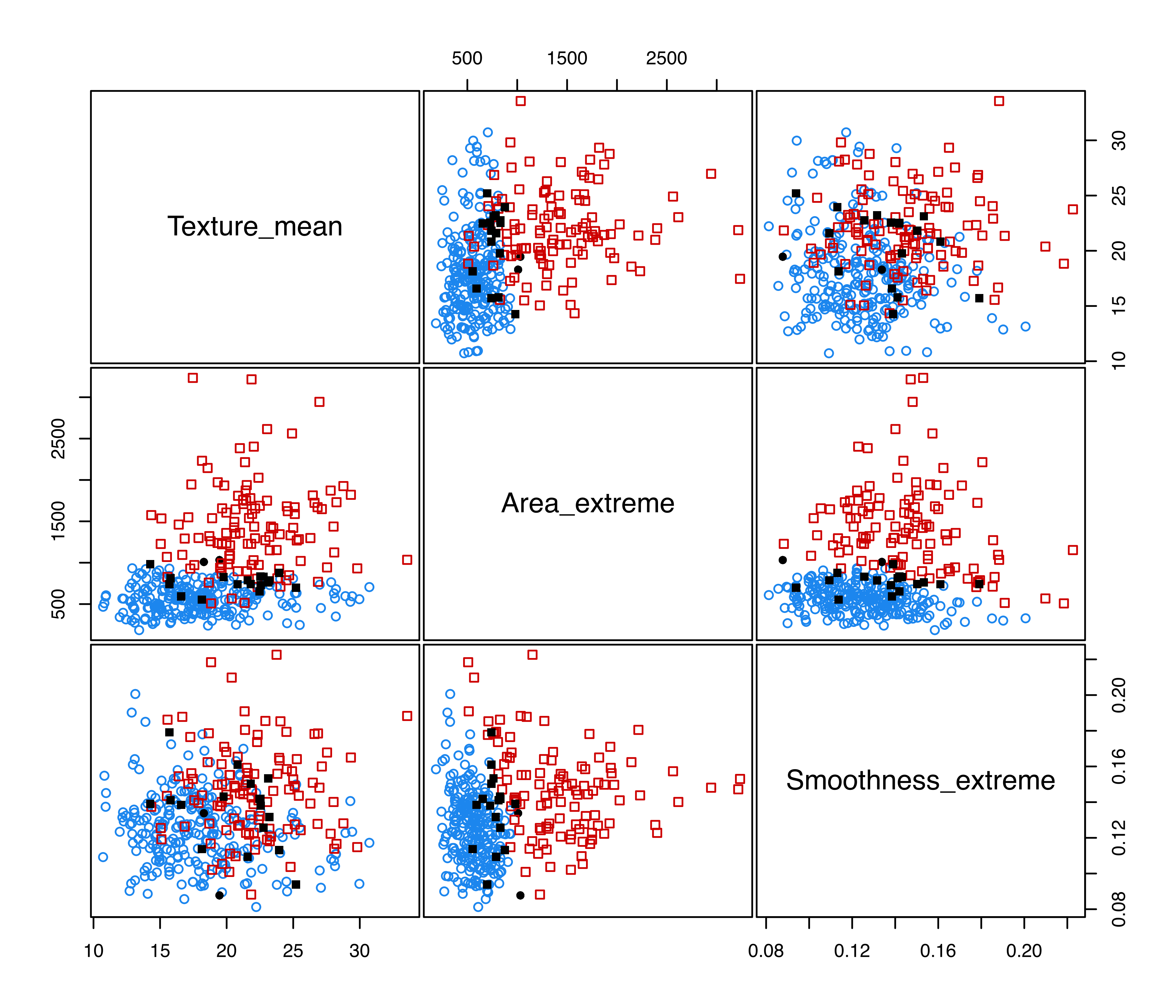
EDDA imposes a single mixture component for each group. However, in certain circumstances, a more flexible model may result in a better classifier. As mentioned in Section 4.2, a more general approach, called MclustDA, is available, in which a finite mixture of Gaussian distributions is used within each class, with both the number of components and covariance matrix structures (expressed following the usual eigen-decomposition in Equation 2.4 allowed to differ among classes. This is the model estimated by default (or by setting modelType = "MclustDA"):
mod2 = MclustDA(X_train, Class_train)
summary(mod2, newdata = X_test, newclass = Class_test)
## ------------------------------------------------
## Gaussian finite mixture model for classification
## ------------------------------------------------
##
## MclustDA model summary:
##
##  log-likelihood   n df     BIC
##         -2893.6 379 27 -5947.5
##
## Classes   n     % Model G
##       B 251 66.23   EEI 3
##       M 128 33.77   EVI 2
##
## Training confusion matrix:
##      Predicted
## Class   B   M
##     B 248   3
##     M   8 120
## Classification error = 0.029
## Brier score          = 0.0262
##
## Test confusion matrix:
##      Predicted
## Class   B   M
##     B 103   3
##     M   5  79
## Classification error = 0.0421
## Brier score          = 0.0273
MclustDA fits a three-component EEI mixture to benign cases, and a two-component EVI mixture to the malignant cases. Note that diagonal covariance structures are used within each class. The training classification error rate is smaller for this model than for the EDDA model. However, the test misclassification rate is the same for the two types of models. This is an effect of overfitting induced by the increased complexity of the MclustDA model, which has 26 parameters to estimate, more than twice the number required by the EDDA model.
Figure 4.4 displays a matrix of pairwise scatterplots between the features showing both the known classes and the estimated mixture components drawn with the code:
plot(mod2, what = "scatterplot")
Specific marginals can be obtained by using the optional argument dimens. For instance, the following code produces the scatterplot for the first two features:
Finally, note that the MDA model of Trevor Hastie and Tibshirani (1996) is equivalent to MclustDA with \(\boldsymbol{\Sigma}_{k} = \lambda\boldsymbol{U}\boldsymbol{\Delta}\boldsymbol{U}{}^{\!\top}\) (model EEE) and fixed \(G_k \ge 1\) for each class. For instance, an MDA model with two mixture components for each class can be fitted using the code:
mod3 = MclustDA(X_train, Class_train, G = 2, modelNames = "EEE")
summary(mod3, newdata = X_test, newclass = Class_test)
## ------------------------------------------------
## Gaussian finite mixture model for classification
## ------------------------------------------------
##
## MclustDA model summary:
##
##  log-likelihood   n df     BIC
##         -2910.8 379 27 -5981.9
##
## Classes   n     % Model G
##       B 251 66.23   EEE 2
##       M 128 33.77   EEE 2
##
## Training confusion matrix:
##      Predicted
## Class   B   M
##     B 247   4
##     M  10 118
## Classification error = 0.0369
## Brier score          = 0.0297
##
## Test confusion matrix:
##      Predicted
## Class   B   M
##     B 104   2
##     M   4  80
## Classification error = 0.0316
## Brier score          = 0.0248
4.4 Evaluating Classifier Performance
Evaluating the performance of a classifier is an essential part of any classification task. Mixture models used for classification are able to generate two types of predictions: the most likely class label according to the MAP rule in Equation 4.3, and the posterior probabilities of class membership from Equation 4.2. mclust automatically computes one performance measure for each type of prediction, namely the misclassification error and the Brier score, to be described in the following sections. Note, however, that several other measures exist, such as the Receiving Operating Characteristic (ROC) curve and the Area Under the [ROC] Curve (AUC) for two-class cases, and it is possible to compute them using the estimates provided by the predict() method associated with MclustDA objects.
4.4.1 Evaluating Predicted Classes: Classification Error
The simplest measure available is the misclassification error rate, or simply the classification error, which is the proportion of wrong predictions made by the classifier: \[ \CE = \frac{1}{n} \sum_{i=1}^n \mathnormal{I}(\widehat{y}_i \ne y_i) , \tag{4.4}\] where \(y_i = \{C_k\}\) is the known class for the \(i\)th observation, \(\widehat{y}_i = \{C_{\widehat{k}}\}\) is the predicted class label, and \(\mathnormal{I}(\widehat{y}_i \ne y_i)\) is an indicator function that equals \(1\) if \(\widehat{y}_i \ne y_i\) and \(0\) otherwise. A good classifier should have a small error rate, preferably close to zero. Equivalently, the accuracy of a classifier is defined as the proportion of correct predictions, \(1 - \CE\). Note, however, that when classes are unbalanced (not represented more or less equally), the error rate or accuracy may not be meaningful. A classifier could have a high overall accuracy yet not be able to accurately detect members of small classes.
4.4.2 Evaluating Class Probabilities: Brier Score
The Brier score is a measure of the predictive accuracy for probabilistic predictions. It is computed as the mean squared difference between the true class indicators and the predicted probabilities.
Based on the original multi-class definition by Brier (1950), the following formula provides the normalized Brier score: \[ \BS = \frac{1}{2n} \sum_{i=1}^n \sum_{k=1}^K (C_{ik} - \widehat{p}_{ik})^2 , \] where \(n\) is the number of observations, \(K\) is the number of classes, \(C_{ik} = 1\) if observation \(i\) is from class \(k\) and 0 otherwise, and \(\widehat{p}_{ik}\) is the predicted probability that observation \(i\) belongs to class \(k\). In this formula, the inclusion of the constant 2 in the denominator ensures that the index takes values in the range \([0,1]\) (Kruppa et al. 2014, Kruppa:etal:2014b).
The Brier score is a strictly proper score (Gneiting and Raftery 2007), which implies that it takes its minimal value only when the predicted probabilities match the empirical probabilities. Thus, small values of the Brier score indicate high prediction accuracy, with \(\BS = 0\) when the observations are all correctly classified with probability one.
4.4.3 Estimating Classifier Performance: Test Set and Resampling-Based Validation
Any performance measure computed using the training set will tend to provide an optimistic performance estimate. For instance, the training classification error rate \(\CE_{\text{train}}\) is obtained by applying Equation 4.4 to the training observations. This measure of the accuracy of a classifier is optimistic because the same set of observations is used for both model estimation and for its assessment. A more realistic estimate can be obtained by computing the test misclassification error rate, which is the error rate computed on a fresh test set of \(m\) observations \(\mathcal{D}_\text{test}= \{(\boldsymbol{x}^*_1,y^*_1), \dots, (\boldsymbol{x}^*_m,y^*_m)\}\): \[
\CE_{\text{test}} = \frac{1}{m} \sum_{i=1}^{m} \mathnormal{I}(y^*_i \ne \widehat{y}^*_i),
\] where \(\widehat{y}^*_i\) is the predicted class label that results from applying the classifier with feature vector \(\boldsymbol{x}^*\).
This seems an obvious choice, “but, to get reasonable precision of the performance values, the size of the test set may need to be large” (Kuhn and Johnson 2013, 66). The same considerations also apply to the Brier score.
In cases where a test set is not available, or its size is not sufficient to guarantee reliable estimates, an assessment of a model’s performance can be obtained by resampling methods. Different resampling schemes are available, but all rely on modeling repeated samples drawn from a training set.
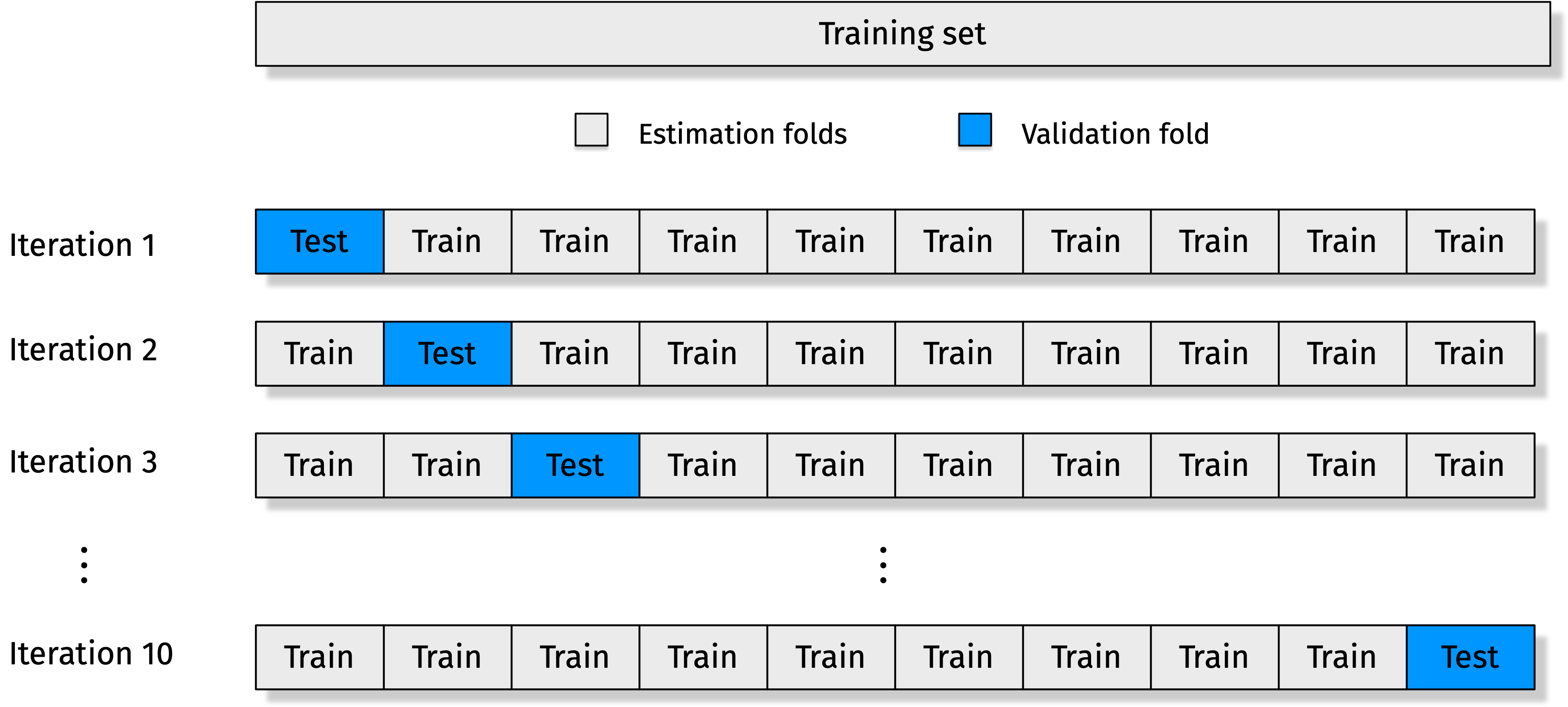
Cross-validation is a simple and intuitive way to obtain a realistic performance measure. A standard resampling scheme is the \(V\)-fold cross-validation approach, which randomly splits the set of training observations into \(V\) parts or folds. At each step of the procedure, data from \(V-1\) folds are used for model fitting, and the held-out fold is used as a validation set. Figure 4.5 provides a schematic view of 10-fold cross-validation.
Consider a generic loss function of the prediction error, say \(L(y,\widehat{y})\), that we would like to minimize. For instance, by setting \(L(y,\widehat{y}) = \mathnormal{I}(y \ne \widehat{y})\), the \(0-1\) loss, we obtain the misclassification error rate, whereas by setting \(L(y,\widehat{y}) = (C_k - \widehat{p})^2\), the squared error with respect to the estimated probability \(\widehat{p}\), we obtain the Brier score. The \(V\)-fold cross-validation steps are the following:
- Split the training set into \(V\) folds of roughly equal size (and stratified1), say \(F_1, \dots, F_V\).
-
For \(v=1, \dots, V\):
fit the model using \(\{(\boldsymbol{x}_i,y_i): i \notin F_v\}\) as training set;
evaluate the model using \(\{(\boldsymbol{x}_i,y_i): i \in F_v\}\) as validating set by computing \[ L_v = \frac{1}{n_v} \sum_{i \in F_v} L(y_i, \widehat{y}_i), \] where \(n_v\) is the number of observations in fold \(F_v\).
Average the loss function over the folds by computing \[ L_{\CV} = \sum_{v = 1}^V \frac{n_v}{n} L_v = \frac{1}{n} \sum_{v = 1}^V \sum_{i \in F_v} L(y_i, \widehat{y}_i). \]
There is no general rule for choosing an optimal value for \(V\). If \(V = n\), the procedure is called leave-one-out cross-validation (LOOCV), because one data point is held out at a time. Large values of \(V\) reduce the bias of the estimator but increase its variance, while small values of \(V\) increase the bias but decrease the variance. Furthermore, for large values of \(V\), the computational burden may be quite high. For these reasons, it is often suggested to set \(V\) equal to 5 or 10 (T. Hastie, Tibshirani, and Friedman 2009, sec. 7.10).
An advantage of using a cross-validation approach is that it provides an estimate of the standard error of the procedure. This can be computed as \[ \se(L_{\CV}) = \frac{\sd(L)}{\sqrt{V}}, \] where \[ \sd(L) = \sqrt{ \frac{\sum_{v=1}^V (L_v - L_{\CV})^2 n_v}{n(V-1)/V} }. \] The estimate \(\se(L_{\CV})\) is often used for implementing the one-standard error rule: when models of different complexity are compared, select the simplest model whose performance is within one standard error of the best value (Breiman et al. 1984, sec. 8.1 and 14.1). For an in-depth investigation of the behavior of cross-validation for some commonly used statistical models, see Bates, Hastie, and Tibshirani (2021).
4.4.4 Cross-Validation in mclust
The function cvMclustDA() is available in mclust to carry out \(V\)-fold cross-validation as discussed above. It requires an object as returned by MclustDA() and, among the optional arguments, nfold can be used to set the number of folds (by default set to 10).
Example 4.2 Evaluation of classification models using cross-validation for the Wisconsin diagnostic breast cancer data
Consider the classification models estimated in Example 4.1. The following code computes the 10-fold CV for the selected EDDA and MclustDA models:
cv1 = cvMclustDA(mod1)
str(cv1)
## List of 6
## $ classification: Factor w/ 2 levels "B","M": 2 1 1 1 1 2 1 1 1 1 ...
## $ z : num [1:379, 1:2] 0.191 0.744 0.972 0.927 0.705 ...
## ..- attr(*, "dimnames")=List of 2
## .. ..$ : NULL
## .. ..$ : chr [1:2] "B" "M"
## $ ce : num 0.0528
## $ se.ce : num 0.0125
## $ brier : num 0.0399
## $ se.brier : num 0.00734
cv2 = cvMclustDA(mod2)
str(cv2)
## List of 6
## $ classification: Factor w/ 2 levels "B","M": 2 1 1 1 2 2 1 1 1 2 ...
## $ z : num [1:379, 1:2] 0.304 0.891 0.916 0.994 0.471 ...
## ..- attr(*, "dimnames")=List of 2
## .. ..$ : NULL
## .. ..$ : chr [1:2] "B" "M"
## $ ce : num 0.0317
## $ se.ce : num 0.00765
## $ brier : num 0.0298
## $ se.brier : num 0.00462
The list of values returned by cvMclustDA() contains the cross-validated predicted classes (classification), the posterior class conditional probabilities (z), followed by the cross-validated metrics (the misclassification error rate and the Brier score) and their standard errors. The latter can be extracted using:
Training and resampling metrics for all of the EDDA models and the MclustDA model can be obtained using the following code:
models = mclust.options("emModelNames")
tab_CE = tab_Brier =
  matrix(as.double(NA), nrow = length(models)+1, ncol = 5)
rownames(tab_CE) = rownames(tab_Brier) =
  c(paste0("EDDA[", models, "]"), "MCLUSTDA")
colnames(tab_CE) = colnames(tab_Brier) =
  c("Train", "10-fold CV", "se(CV)", "lower", "upper")
for (i in seq(models))
{
  mod = MclustDA(X, Class, modelType = "EDDA",
                  modelNames = models[i], verbose = FALSE)
  pred = predict(mod, X)
  cv = cvMclustDA(mod, nfold = 10, verbose = FALSE)
  #
  tab_CE[i, 1] = classError(pred$classification, Class)$errorRate
  tab_CE[i, 2] = cv$ce
  tab_CE[i, 3] = cv$se.ce
  tab_CE[i, 4] = cv$ce - cv$se.ce
  tab_CE[i, 5] = cv$ce + cv$se.ce
  #
  tab_Brier[i, 1] = BrierScore(pred$z, Class)
  tab_Brier[i, 2] = cv$brier
  tab_Brier[i, 3] = cv$se.brier
  tab_Brier[i, 4] = cv$brier - cv$se.brier
  tab_Brier[i, 5] = cv$brier + cv$se.brier
}
i = length(models)+1
mod = MclustDA(X, Class, modelType = "MclustDA", verbose = FALSE)
pred = predict(mod, X)
cv = cvMclustDA(mod, nfold = 10, verbose = FALSE)
#
tab_CE[i, 1] = classError(pred$classification, Class)$errorRate
tab_CE[i, 2] = cv$ce
tab_CE[i, 3] = cv$se.ce
tab_CE[i, 4] = cv$ce - cv$se.ce
tab_CE[i, 5] = cv$ce + cv$se.ce
#
tab_Brier[i, 1] = BrierScore(pred$z, Class)
tab_Brier[i, 2] = cv$brier
tab_Brier[i, 3] = cv$se.brier
tab_Brier[i, 4] = cv$brier - cv$se.brier
tab_Brier[i, 5] = cv$brier + cv$se.brier
The following table gives the training error, the 10-fold CV error with its standard error, and the lower and upper bounds computed as \(\pm\) one standard error from the CV estimate:
tab_CE
##              Train 10-fold CV    se(CV)    lower    upper
## EDDA[EII] 0.112478   0.117750 0.0168034 0.100947 0.134554
## EDDA[VII] 0.079086   0.079086 0.0120644 0.067022 0.091150
## EDDA[EEI] 0.087873   0.087873 0.0089230 0.078950 0.096797
## EDDA[VEI] 0.091388   0.093146 0.0128794 0.080266 0.106025
## EDDA[EVI] 0.066784   0.072056 0.0083953 0.063661 0.080452
## EDDA[VVI] 0.043937   0.047452 0.0064740 0.040978 0.053926
## EDDA[EEE] 0.066784   0.068541 0.0076137 0.060928 0.076155
## EDDA[VEE] 0.072056   0.073814 0.0159524 0.057861 0.089766
## EDDA[EVE] 0.059754   0.065026 0.0073839 0.057642 0.072410
## EDDA[VVE] 0.042179   0.043937 0.0088144 0.035122 0.052751
## EDDA[EEV] 0.047452   0.050967 0.0075542 0.043412 0.058521
## EDDA[VEV] 0.052724   0.056239 0.0108316 0.045407 0.067071
## EDDA[EVV] 0.045694   0.047452 0.0074344 0.040017 0.054886
## EDDA[VVV] 0.036907   0.038664 0.0090412 0.029623 0.047705
## MCLUSTDA  0.022847   0.036907 0.0105586 0.026348 0.047465
The same information is also shown graphically in Figure 4.6 using:
library("ggplot2")
df = data.frame(rownames(tab_CE), tab_CE)
colnames(df) = c("model", "train", "cv", "se", "lower", "upper")
df$model = factor(df$model, levels = rev(df$model))
ggplot(df, aes(x = model, y = cv, ymin = lower, ymax = upper)) +
  geom_point(aes(shape = "s1", color = "c1")) +
  geom_errorbar(width = 0.5, col = "dodgerblue3") +
  geom_point(aes(y = train, shape = "s2", color = "c2")) +
  scale_y_continuous(breaks = seq(0, 0.2, by = 0.01), lim = c(0, NA)) +
  scale_color_manual(name = "",
                     breaks = c("c1", "c2"),
                     values = c("dodgerblue3", "black"),
                     labels = c("CV", "Train")) +
  scale_shape_manual(name = "",
                     breaks = c("s1", "s2"),
                     values = c(19, 0),
                     labels = c("CV", "Train")) +
  ylab("Classification error") + xlab("") + coord_flip() +
  theme(legend.position = "top")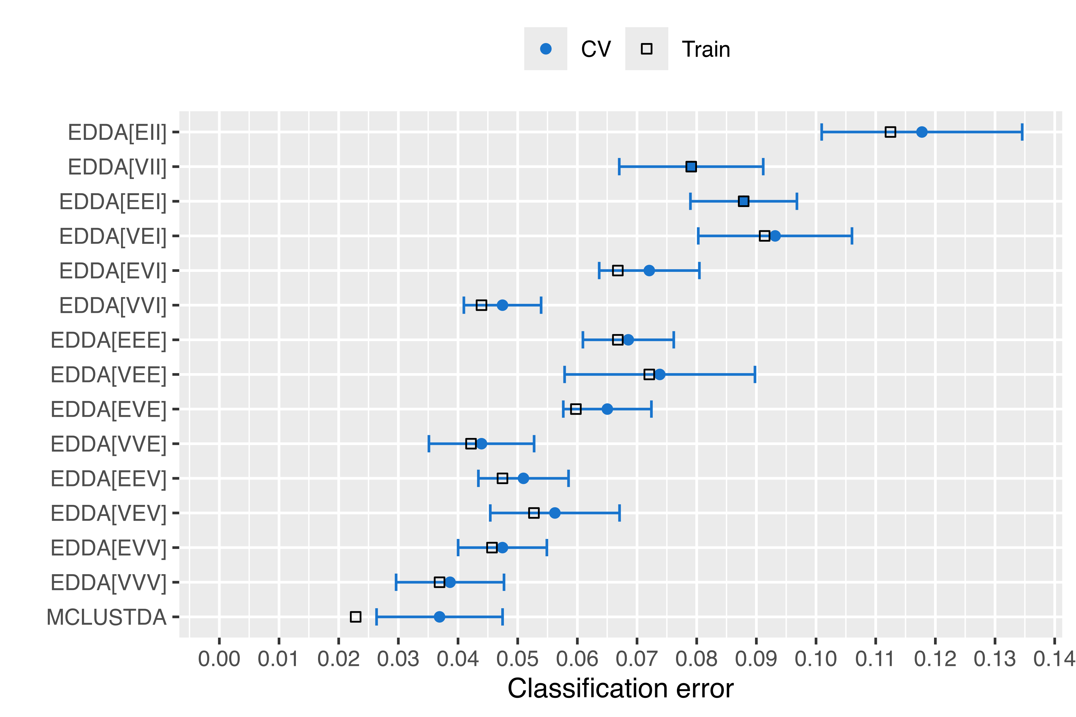
The analogous table for the Brier score is:
tab_Brier
##              Train 10-fold CV    se(CV)    lower    upper
## EDDA[EII] 0.095691   0.096282 0.0141399 0.082142 0.110422
## EDDA[VII] 0.072572   0.072936 0.0099342 0.063001 0.082870
## EDDA[EEI] 0.055086   0.055573 0.0055047 0.050068 0.061078
## EDDA[VEI] 0.060386   0.062123 0.0094198 0.052703 0.071543
## EDDA[EVI] 0.047277   0.049384 0.0067815 0.042603 0.056166
## EDDA[VVI] 0.036197   0.037103 0.0044475 0.032655 0.041550
## EDDA[EEE] 0.051470   0.052056 0.0040711 0.047984 0.056127
## EDDA[VEE] 0.052813   0.054901 0.0085825 0.046318 0.063483
## EDDA[EVE] 0.043315   0.046130 0.0053728 0.040757 0.051502
## EDDA[VVE] 0.035243   0.035845 0.0065776 0.029268 0.042423
## EDDA[EEV] 0.039127   0.040170 0.0040287 0.036141 0.044199
## EDDA[VEV] 0.041625   0.043191 0.0074828 0.035708 0.050674
## EDDA[EVV] 0.036139   0.037555 0.0050249 0.032530 0.042580
## EDDA[VVV] 0.028803   0.030183 0.0063246 0.023859 0.036508
## MCLUSTDA  0.022999   0.026530 0.0064555 0.020075 0.032986
with the corresponding plot in Figure 4.7:
df = data.frame(rownames(tab_Brier), tab_Brier)
colnames(df) = c("model", "train", "cv", "se", "lower", "upper")
df$model = factor(df$model, levels = rev(df$model))
ggplot(df, aes(x = model, y = cv, ymin = lower, ymax = upper)) +
  geom_point(aes(shape = "s1", color = "c1")) +
  geom_errorbar(width = 0.5, col = "dodgerblue3") +
  geom_point(aes(y = train, shape = "s2", color = "c2")) +
  scale_y_continuous(breaks = seq(0, 0.2, by = 0.01), lim = c(0, NA)) +
  scale_color_manual(name = "",
                     breaks = c("c1", "c2"),
                     values = c("dodgerblue3", "black"),
                     labels = c("CV", "Train")) +
  scale_shape_manual(name = "",
                     breaks = c("s1", "s2"),
                     values = c(19, 0),
                     labels = c("CV", "Train")) +
  ylab("Brier score") + xlab("") + coord_flip() +
  theme(legend.position = "top")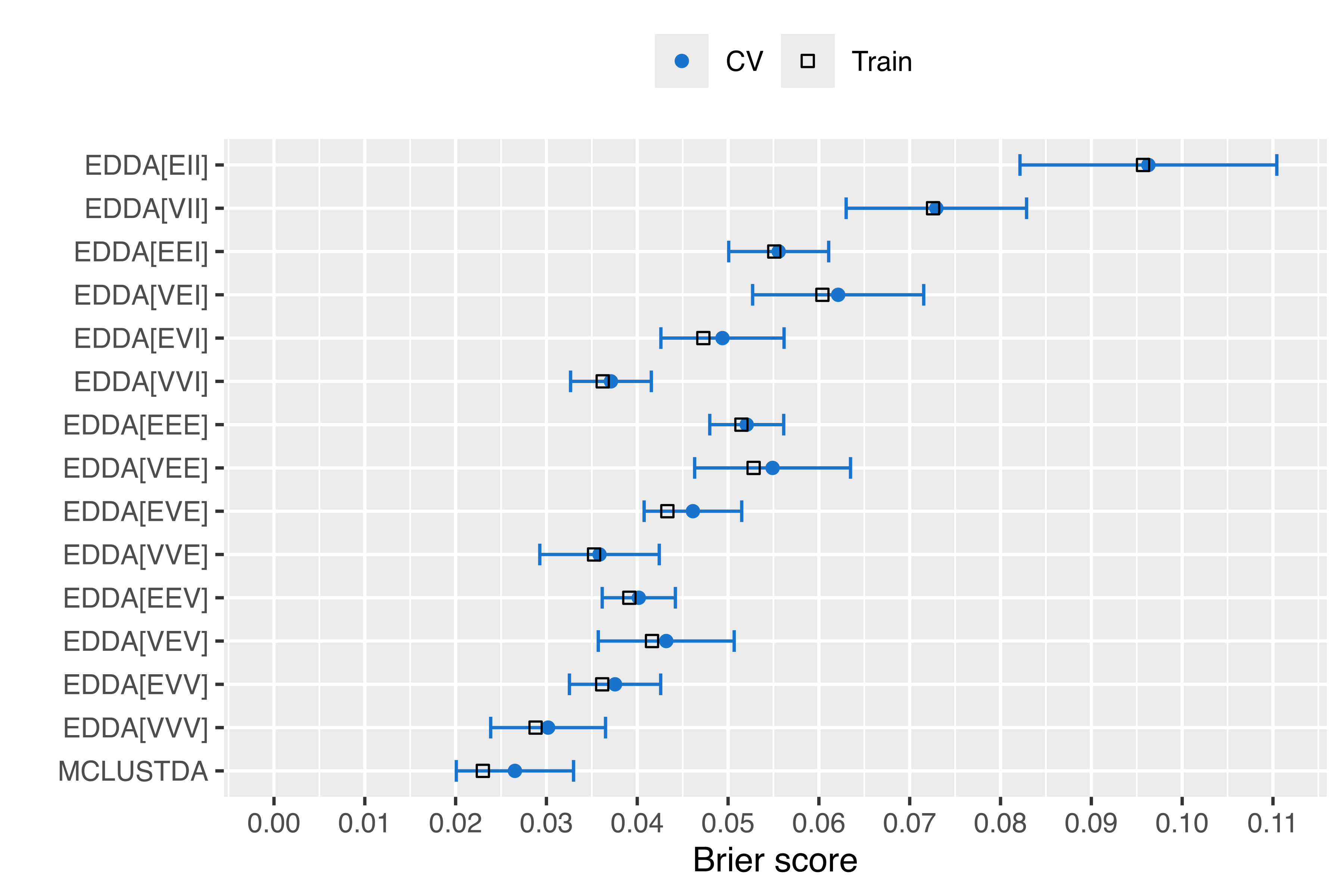
The plots in Figure 4.6 and Figure 4.7 show that, by increasing the complexity of the model, it is sometimes possible to improve the accuracy of the predictions. In particular, the MclustDA model had better performance than the EDDA models, with the exception of the EDDA model with unconstrained covariances (VVV), which had both misclassification error rate and Brier score within one standard error from the best.
The information returned by cvMclustDA() can also be used for computing other cross-validation metrics. For instance, in the binary class case two popular measures are sensitivity and specificity. The sensitivity, or true positive rate, is given by the ratio of the number observations that are classified in the positive class to the total number of positive cases. The specificity, or true negative rate, is given by the ratio of observations that are classified in the negative class to the total number of negative cases. Both metrics are easily computed from the confusion matrix, obtained by cross-tabulating the true classes and the classes predicted by a classifier.
Example 4.3 ROC-AUC analysis of classification models for the Wisconsin diagnostic breast cancer data
Returning to the Wisconsin diagnostic breast cancer data in Example 4.1, we are mainly interested in the identification of patients with malignant diagnosis, so the positive class can be taken to be class M, while benign cases (B) are assigned to the negative class.
The code above uses the cross-validated classifications obtained using the MAP approach, which for the binary class case is equivalent to setting the classification probability threshold at \(0.5\). However, the posterior probabilities returned by cvMclustDA() can be used to get classifications at different threshold values. The following code computes the sensitivity and specificity over a fine grid of threshold values:
threshold = seq(0, 1, by = 0.01)
sensitivity = specificity = rep(NA, length(threshold))
for(i in 1:length(threshold))
{
pred = factor(ifelse(cv1$z[, "M"] > threshold[i], "M", "B"),
levels = c("B", "M"))
tab = table(pred, Class_train)
sensitivity[i] = tab[2, 2]/sum(tab[, 2])
specificity[i] = tab[1, 1]/sum(tab[, 1])
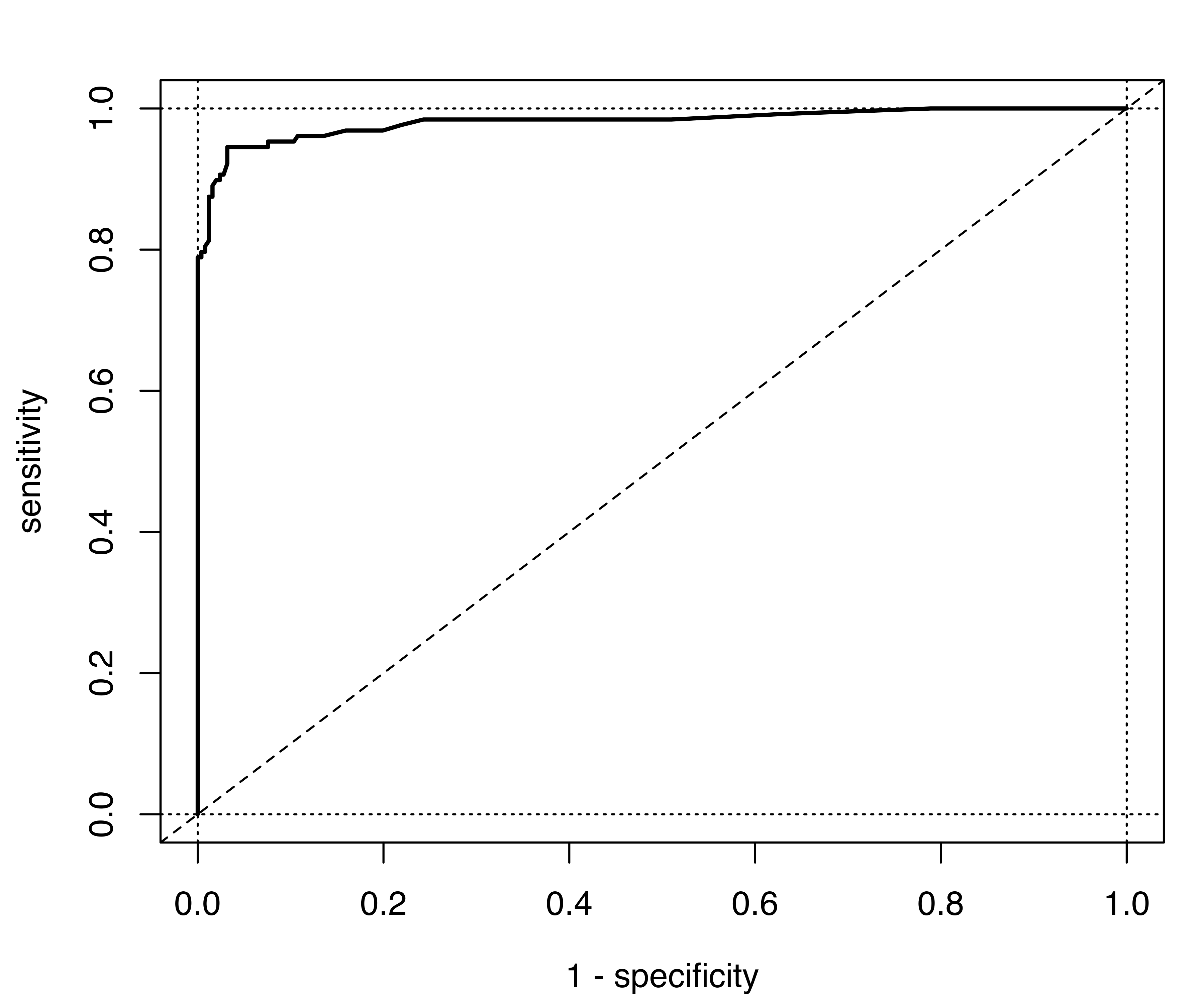
}The metrics computed above for varying thresholds in binary decisions can be represented graphically using the Receiver Operating Characteristic (ROC) curve, which plots the sensitivity (true positive rate) vs. one minus the specificity (false positive rate). The resulting display is shown in Figure 4.8 (a) and obtained with the following code:
Notice that the optimal ROC curve would pass through the upper left corner, which corresponds to both sensitivity and specificity equal to 1.
A summary of the ROC curve which is used for evaluating the overall performance of a classifier is the Area Under the Curve (AUC). This is equal to 1 for a perfect classifier, and 0.5 for a random classification; values larger than 0.8 are considered to be good (Lantz 2019, 333). Provided that the threshold grid is fine enough, a simple approximation of the AUC is obtained using the following function:
The value of AUC indicates a classifier with a very good classification performance.
The same ROC-AUC analysis can also be replicated for the selected MclustDA model (in object mod2), producing the ROC curve shown in Figure 4.8 (b). The corresponding value of the AUC is 0.98506.

Finally, the ROC curve can also be used to select an optimal threshold value. This can be set at the value where the true positive rate is high and the false positive rate is low, which is equivalent to maximizing Youden’s index: \[ J = \text{Sensitivity} - (1 - \text{Specificity}) = \text{Sensitivity} + \text{Specificity} - 1. \] Note that \(J\) corresponds to the vertical distance between the ROC curve and the random classification line. The following code computes Youden’s index and the optimal threshold for the selected EDDA model:
ROC curves are a suitable measure of performance when the distribution of the two classes is approximately equal. Otherwise, Precision-Recall (PR) curves are a better alternative. Both measures require a sufficient number of thresholds to obtain an accurate estimate of the corresponding area under the curve. A discussion of the relationship between ROC and PR curves can be found in Davis and Goadrich (2006). R implementations include CRAN package PRROC (Keilwagen, Grosse, and Grau 2014; Grau, Grosse, and Keilwagen 2015) and ROCR (Sing et al. 2005).
4.5 Classification with Unequal Costs of Misclassification
In many practical applications, different costs are associated with different types of classification error. Thus it can be argued that the decision rule should be based on the principle that the total cost of misclassification should be minimized. Costs can be incorporated into a decision rule either at the learning stage or at the prediction stage.
We now describe a strategy for Gaussian mixtures that takes costs into account only at the final prediction stage. Let \(c(k|j)\) be the cost of allocating an observation from class \(j\) to class \(k \ne j\), with \(c(j|j) = 0\). Let \(p(k|j) = \Pr(C_k | \boldsymbol{x}\in C_j)\) be the probability of allocating an observation coming from class \(j\) to class \(k\). The expected cost of misclassification (ECM) for class \(j\) is given by \[ \ECM(j) = \sum_{k \ne j}^K c(k|j) p(k|j) \propto \sum_{k \ne j}^K c(k|j) \tau_k f(\boldsymbol{x}| C_k), \] and the overall ECM is thus \[ \ECM = \sum_{j=1}^K \ECM(j) = \sum_{j=1}^K \sum_{k \ne j}^K c(k|j) p(k|j). \] According to this criterion, a new observation \(\boldsymbol{x}\) should be allocated by minimizing the expected cost of misclassification.
In the case of equal costs of misclassification (\(c(k|j) = 1\) if \(k \ne j\)), we obtain \[ \ECM(j) = \sum_{k \ne j}^K p(k|j) \propto \sum_{k \ne j}^K \tau_k f(\boldsymbol{x}| C_k), \] and we allocate an observation \(\boldsymbol{x}\) to the class \(C_k\) that minimizes \(\ECM(j)\), or, equivalently, that maximizes \(\tau_k f(\boldsymbol{x}| C_k)\). This rule is the same as the standard MAP rule which uses the posterior probability from Equation 4.2.
In the case of unequal costs of misclassification, consider the \(K \times K\) matrix of costs having the form: \[ C = \{ c(k|j) \} = \begin{bmatrix} 0 & c(2|1) & c(3|1) & \dots & c(K|1) \\ c(1|2) & 0 & c(3|2) & \dots & c(K|2) \\ c(1|3) & c(2|3) & 0 & \dots & c(K|3) \\ \vdots & \vdots & \ddots & \vdots & \vdots \\ c(1|K) & c(2|K) & c(3|K) & \dots & 0 \\ \end{bmatrix} . \] A simple solution can be obtained if we assume a constant cost of misclassifying an observation from class \(j\), irrespective of the class predicted. Following (Breiman et al. 1984, 112–15), we can compute the per-class cost \(c(k|j) = c(j)\) for \(j \neq k\), and then get the predictions as in the unit-cost case with adjusted prior probabilities for the classes: \[ \tau^*_j = \frac{c(j)\tau_j}{\displaystyle\sum_{j=1}^K c(j)\tau_j}. \] Note that for two-class problems the use of the per-class cost vector is equivalent to using the original cost matrix.
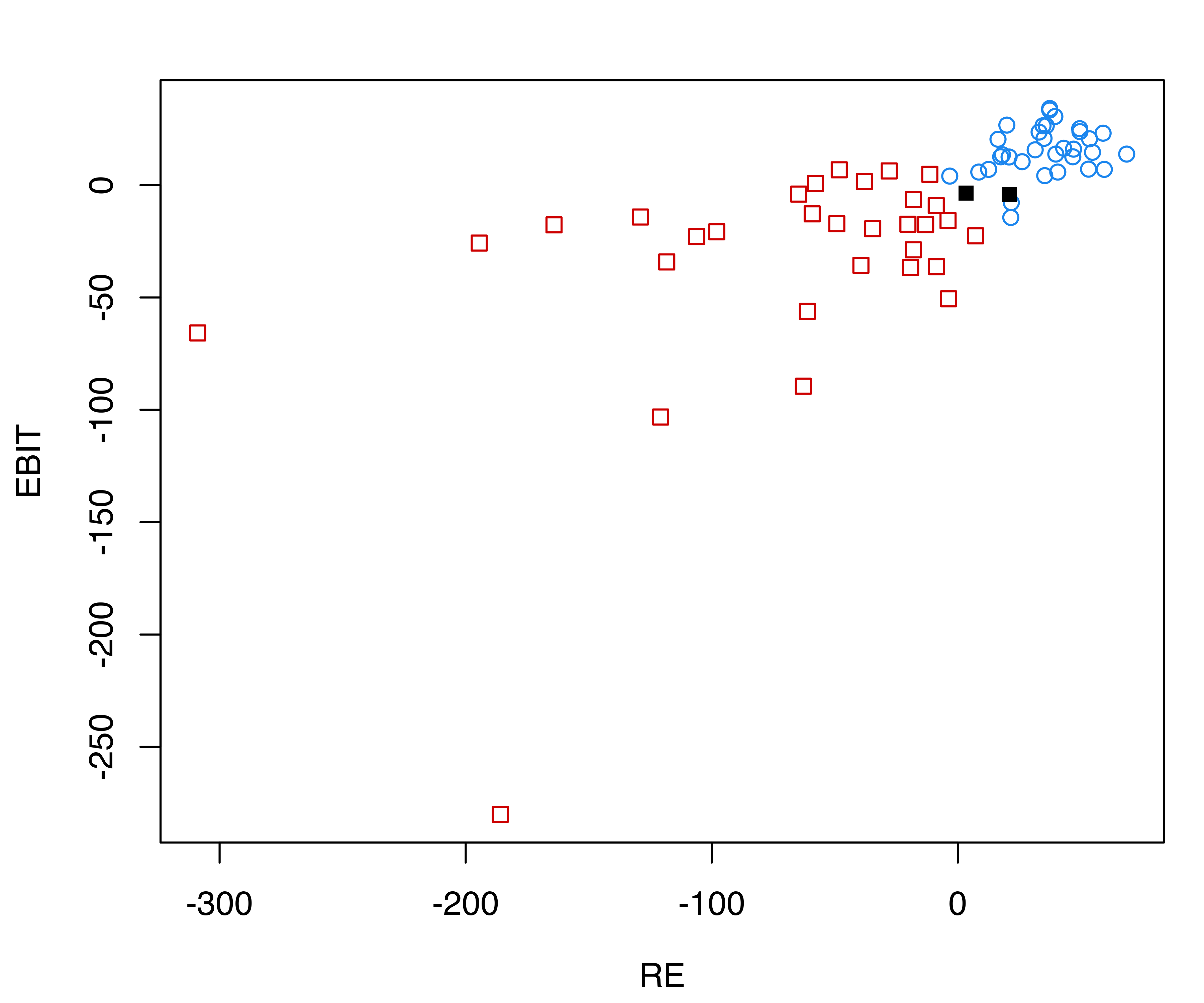
Example 4.4 Bankruptcy prediction based on financial ratios of corporations
Consider the data on financial ratios from Altman (1968), and available in the R package MixGHD (Tortora et al. 2022), which provides the ratio of retained earnings (RE) to total assets, and the ratio of earnings before interests and taxes (EBIT) to total assets, for 66 American corporations, of which half had filed for bankruptcy.
The following code loads the data and plots the financial ratios conditional on the class (see Figure 4.9):
data("bankruptcy", package = "MixGHD")
X = bankruptcy[, -1]
Class = factor(bankruptcy$Y, levels = c(1:0),
               labels = c("solvent", "bankrupt"))
cl = clPairs(X, Class)
legend("bottomright", legend = cl$class,
       pch = cl$pch, col = cl $col, inset = 0.02)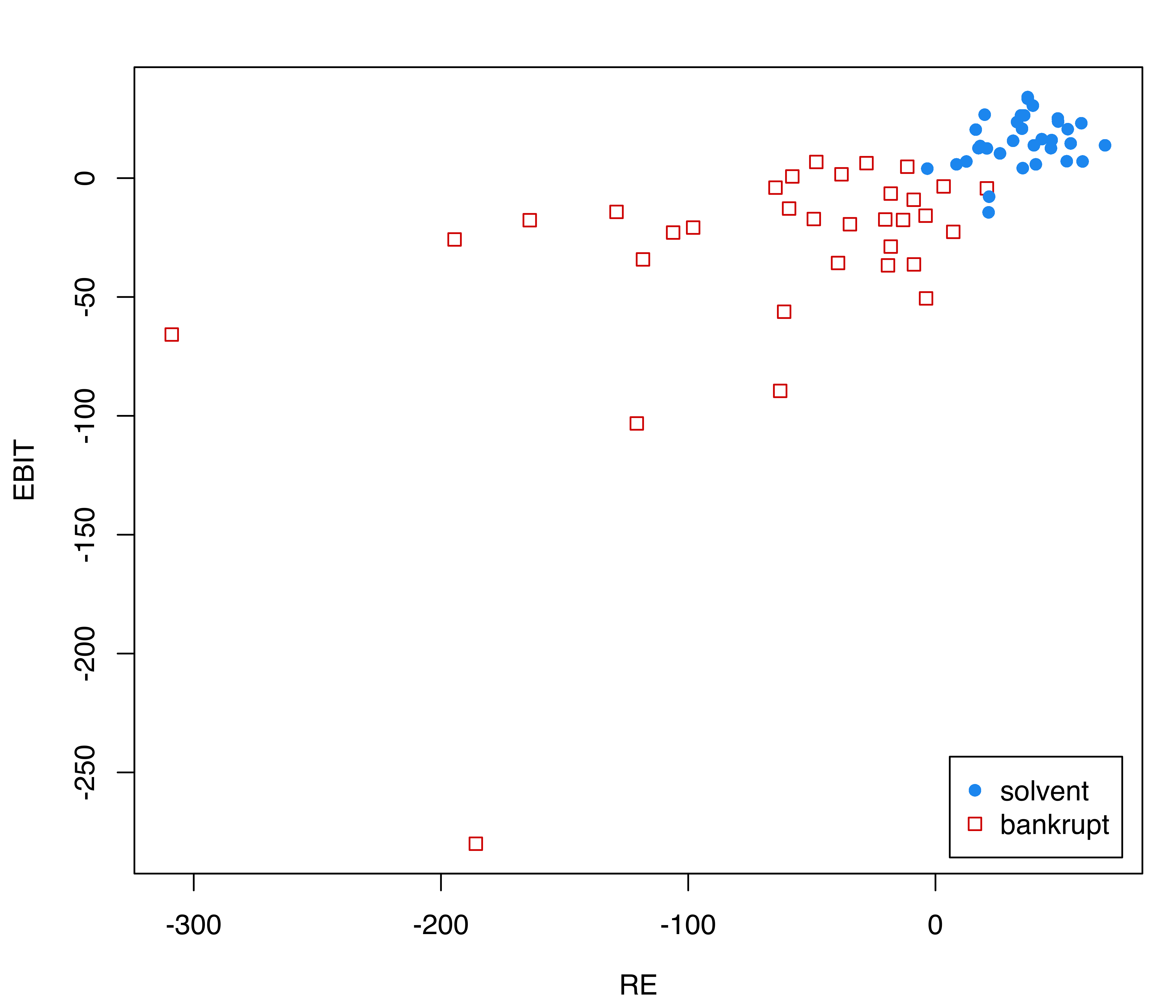
Although the within-class distribution is clearly not Gaussian, in particular for the companies that have declared bankruptcy, we fit an EDDA classification model:
mod = MclustDA(X, Class, modelType = "EDDA")
summary(mod)
## ------------------------------------------------
## Gaussian finite mixture model for classification
## ------------------------------------------------
##
## EDDA model summary:
##
## log-likelihood n df BIC
## -661.27 66 9 -1360.3
##
## Classes n % Model G
## solvent 33 50 VEE 1
## bankrupt 33 50 VEE 1
##
## Training confusion matrix:
## Predicted
## Class solvent bankrupt
## solvent 33 0
## bankrupt 2 31
## Classification error = 0.0303
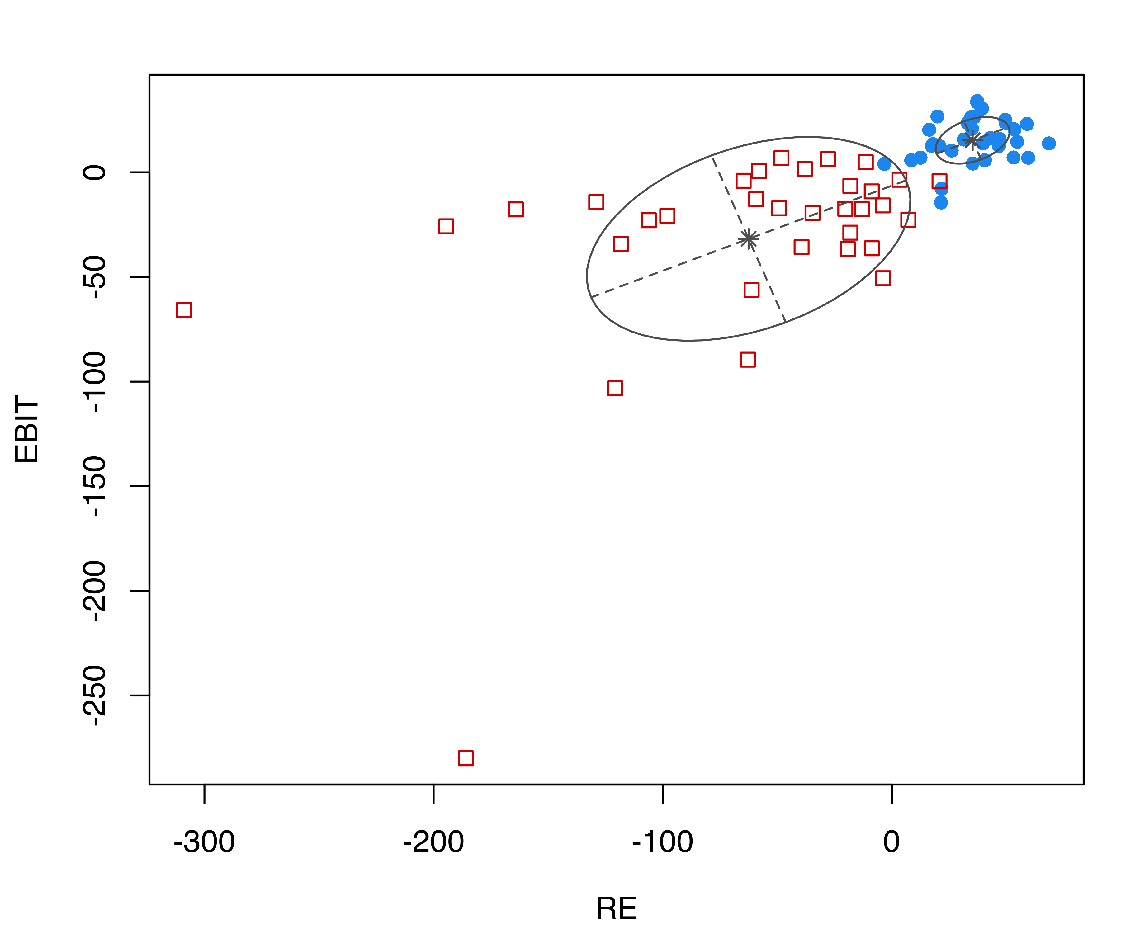
## Brier score = 0.0295The confusion matrix indicates that two training data points are misclassified. Both are bankrupt firms which have been classified as solvent. The following plots show the distribution of financial ratios with (a) Gaussian ellipses implied by the estimated model, and (b) black points corresponding to the misclassified observations (see Figure 4.10):
Now consider the error of misclassifying a bankrupt firm as solvent to be more serious than the opposite. We quantify these different costs of misclassification in a matrix \(C\)
and obtain the per-class cost vector:
rowSums(C)
## [1]  1 10
The total cost of misclassification for the MAP predictions is
Unequal costs of misclassification can be included in the prediction as follows:
The last command shows that we have been able to reduce the total cost by zeroing out the errors for bankrupt firms, at the same time increasing the errors for solvent corporations.
4.6 Classification with Unbalanced Classes
Most classification datasets are not balanced; that is, classes have unequal numbers of instances. Small differences between the number of instances in different classes can usually be ignored. In some cases, however, the imbalance in class proportions can be dramatic, and the class of interest is sometimes the class with the smallest number of cases. For instance, in studies aimed at identifying fraudulent transactions, classes are typically unbalanced, with the vast majority of the transactions not being fraudulent. In medical studies aimed at characterizing rare diseases, the class of individuals with the disease is only a small fraction of the total population (the prevalence).
In such situations, a case-control sampling scheme can be adopted by sampling approximately 505 of the data from the cases (fraudulent transactions, individuals suffering from a disease) and 50% from the controls. Balanced datasets can also be obtained in observational studies by undersampling, or downsizing the majority class by removing observations at random until the dataset is balanced. In both cases the class prior probabilities estimated from the training set do not reflect the “true” a priori probabilities. As a result, the predicted posterior class probabilities are not well estimated, resulting in a loss of classification accuracy compared to a classifier based on the true prior probabilities for the classes.
Example 4.5 Classification of synthetic unbalanced two-class data
As an example, consider a simulated binary classification task, with the majority class having distribution \(x | (y = 0) \sim N(0, 1)\), whereas the distribution of the minority class is \(x | (y = 1) \sim N(3, 1)\), and in the population the latter accounts for 10% of cases. Suppose that a training sample is obtained using case-control sampling, so that the two groups have about the same proportion of cases.
A synthetic dataset from this specification can be simulated with the following code and shown graphically in Figure 4.11:
# generate training data from a balanced case-control sample
n_train = 1000
class_train = factor(sample(0:1, size = n_train, prob = c(0.5, 0.5),
replace = TRUE))
x_train = ifelse(class_train == 1, rnorm(n_train, mean = 3, sd = 1),
rnorm(n_train, mean = 0, sd = 1))
hist(x_train[class_train == 0], breaks = 11, xlim = range(x_train),
main = "", xlab = "x",
col = adjustcolor("dodgerblue2", alpha.f = 0.5), border = "white")
hist(x_train[class_train == 1], breaks = 11, add = TRUE,
col = adjustcolor("red3", alpha.f = 0.5), border = "white")
box()
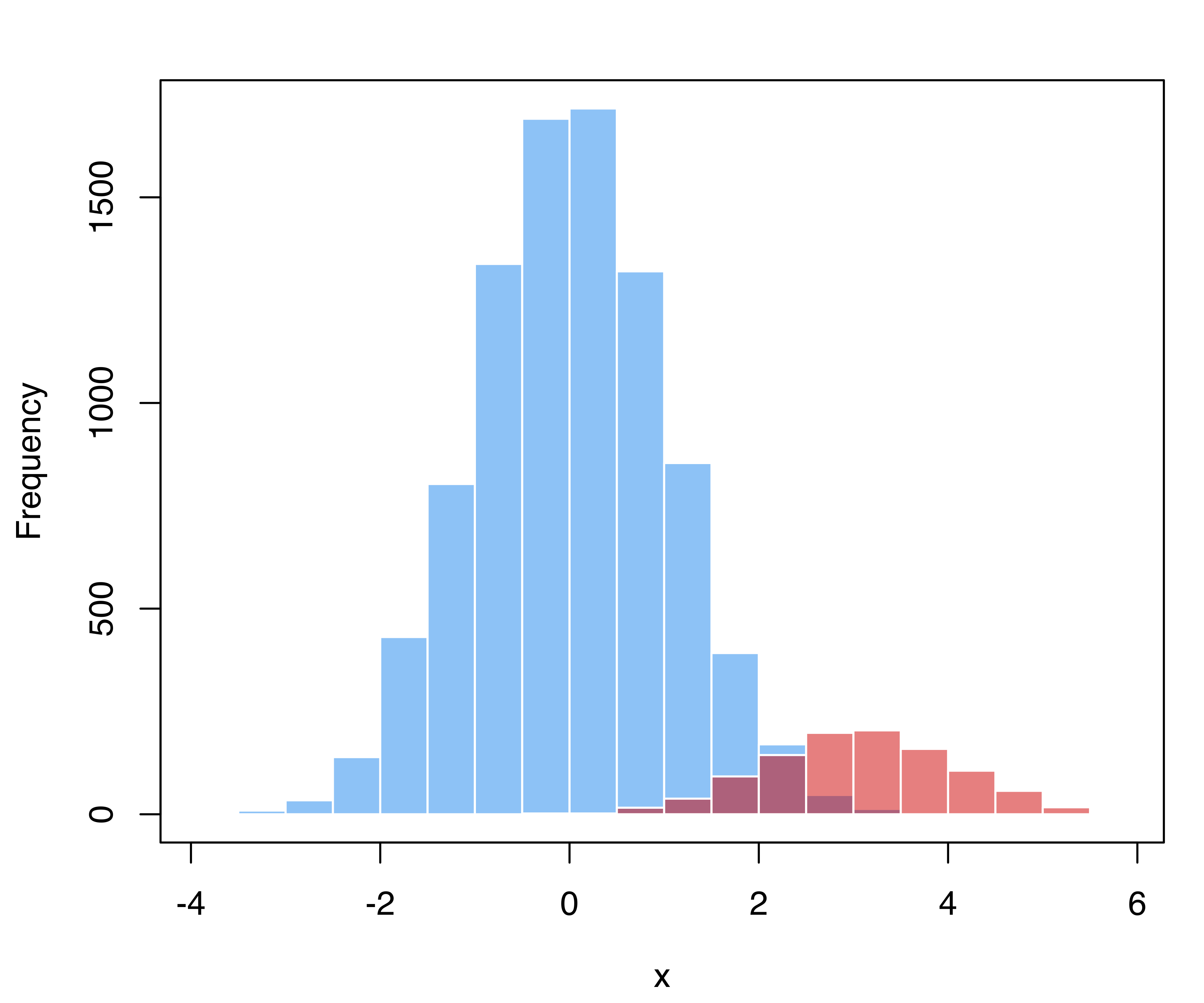
# generate test data from mixture f(x) = 0.9 * N(0,1) + 0.1 * N(3,1)
n = 10000
mixpro = c(0.9, 0.1)
class_test = factor(sample(0:1, size = n, prob = mixpro,
replace = TRUE))
x_test = ifelse(class_test == 1, rnorm(n, mean = 3, sd = 1),
rnorm(n, mean = 0, sd = 1))
hist(x_test[class_test == 0], breaks = 15, xlim = range(x_test),
main = "", xlab = "x",
col = adjustcolor("dodgerblue2", alpha.f = 0.5), border = "white")
hist(x_test[class_test == 1], breaks = 11, add = TRUE,
col = adjustcolor("red3", alpha.f = 0.5), border = "white")
box()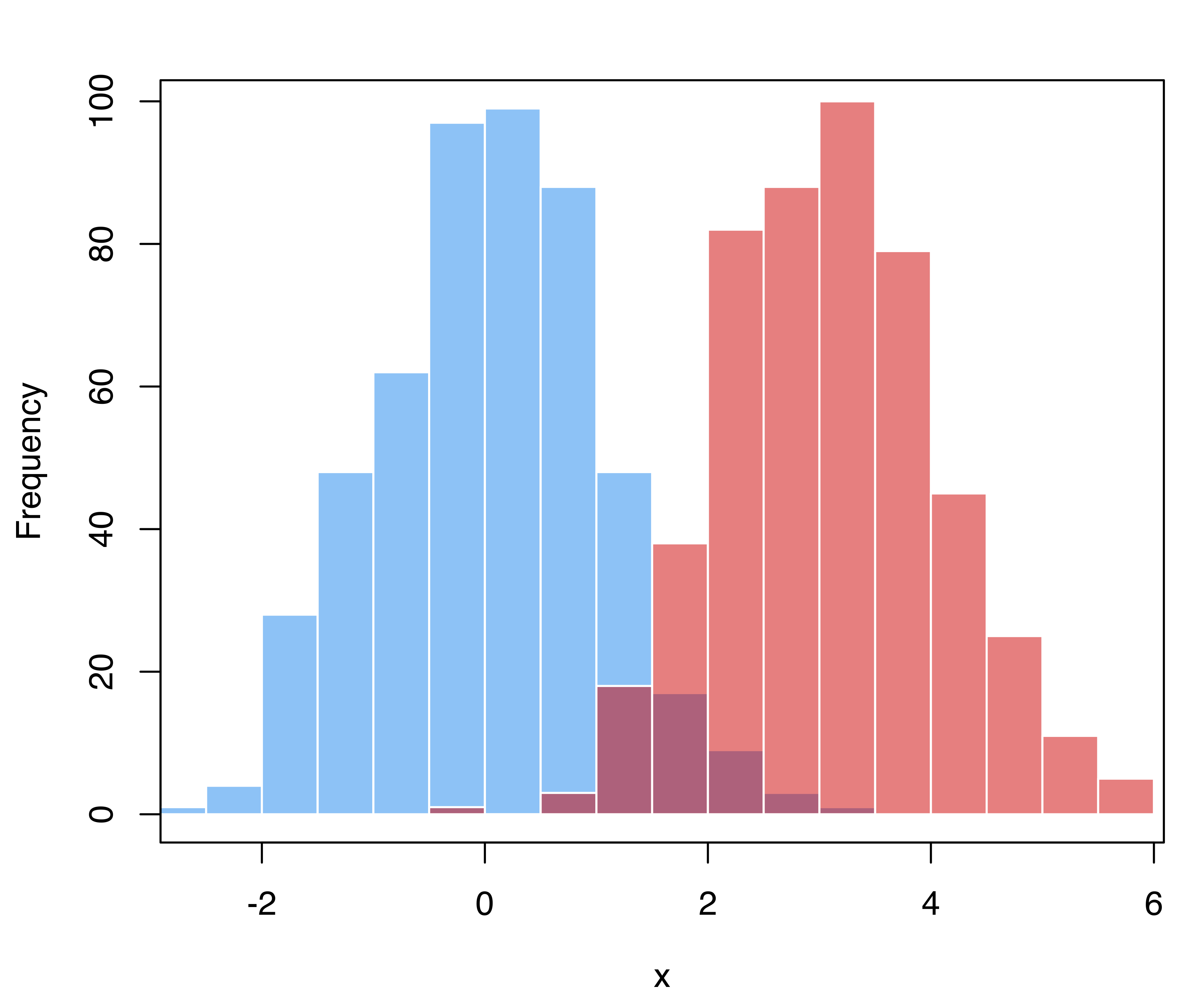
Using the training sample we can estimate a classification Gaussian mixture model:
mod = MclustDA(x_train, class_train)
summary(mod, parameters = TRUE)
## ------------------------------------------------
## Gaussian finite mixture model for classification
## ------------------------------------------------
##
## MclustDA model summary:
##
##  log-likelihood    n df     BIC
##         -1947.1 1000  5 -3928.8
##
## Classes   n    % Model G
##       0 505 50.5     X 1
##       1 495 49.5     X 1
##
## Class prior probabilities:
##     0     1
## 0.505 0.495
##
## Class = 0
##
## Mixing probabilities: 1
##
## Means:
## [1] 0.043067
##
## Variances:
## [1] 0.93808
##
## Class = 1
##
## Mixing probabilities: 1
##
## Means:
## [1] 3.0959
##
## Variances:
## [1] 0.96652
##
## Training confusion matrix:
##      Predicted
## Class   0   1
##     0 479  26
##     1  24 471
## Classification error = 0.05
## Brier score          = 0.0402
The estimated parameters for the class conditional distributions are close to the true values, but the prior class probabilities are highly biased due to the sampling scheme adopted. Performance measures can be computed for the test set:
pred = predict(mod, newdata = x_test)
classError(pred$classification, class_test)$error
## [1] 0.0592
BrierScore(pred$z, class_test)
## [1] 0.045927
showing that they are slightly worse than those for the training set, as is often the case.
For such simulated data we know the true classes, so we can compute the performance measures over a grid of values of the prior probability of the minority class:
The following code produces Figure 4.12, which shows the classification error and the Brier score as functions of the prior probability for the minority class.
matplot(priorProp, cbind(CE, BS), type = "l", lty = 1, lwd = 2, xaxt = "n",
        xlab = "Class prior probability", ylab = "", ylim = c(0, max(CE, BS)),
        col = c("red3", "dodgerblue3"),
        panel.first =
          { abline(h = seq(0, 1, by = 0.05), col = "grey", lty = 3)
            abline(v = seq(0, 1, by = 0.05), col = "grey", lty = 3)
          })
axis(side = 1, at = seq(0, 1, by = 0.1))
abline(v = mod$prop[2],             # training proportions
       lty = 2, lwd = 2)
abline(v = mean(class_test == 1),   # test proportions (usually unknown)
       lty = 3, lwd = 2)
legend("topleft", legend = c("ClassError", "BrierScore"),
       col = c("red3", "dodgerblue3"), lty = 1, lwd = 2, inset = 0.02)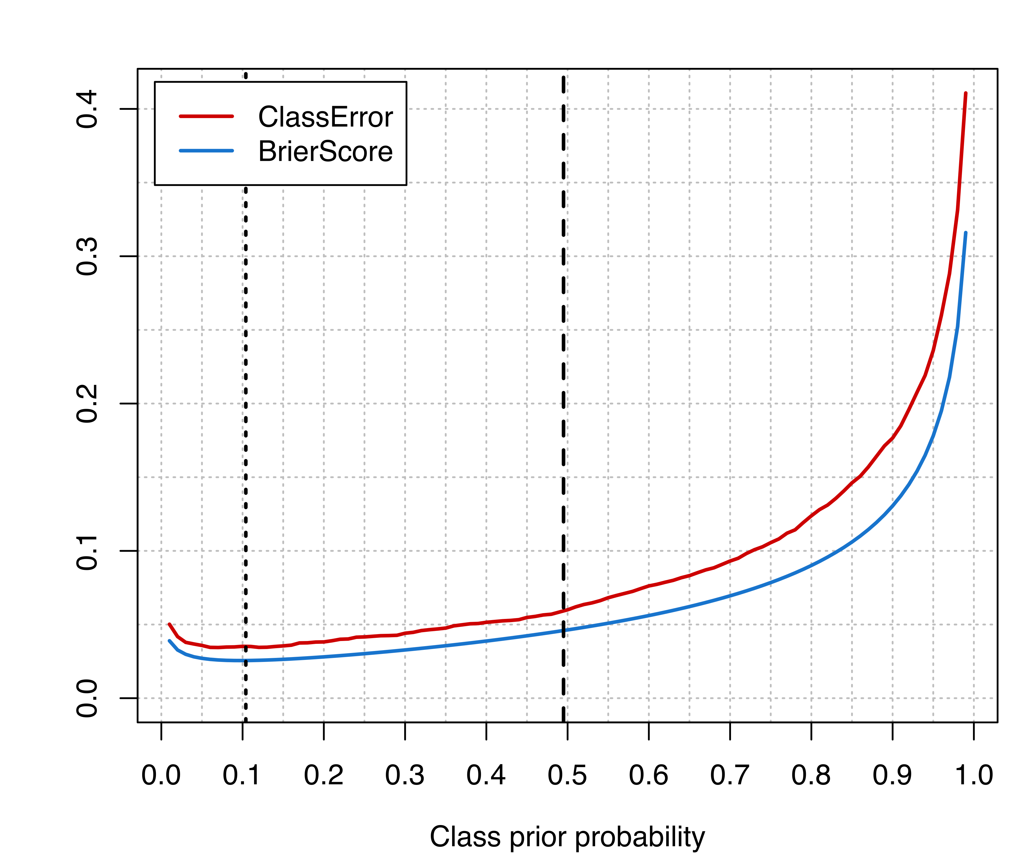
Vertical lines are drawn at the proportion for the minority class in the training set (dashed line), and at the proportion computed on the test set (dotted lines). However, the latter is usually unknown, but the plot clearly shows that there is room for improving the classification accuracy by using an unbiased estimate of the class prior probabilities.
To solve this problem, Saerens, Latinne, and Decaestecker (2002) proposed an EM algorithm that aims at estimating the adjusted posterior conditional probabilities of a classifier, and, as a by-product, provides estimates of the prior class probabilities. This method can be easily adapted to classifiers based on Gaussian mixtures.
Suppose a Gaussian mixture of the type in Equation 4.1 is estimated on the training set \(\mathcal{D}_\text{train}= \{(\boldsymbol{x}_1, y_1), \dots, (\boldsymbol{x}_n, y_n)\}\), and a new test set \(\mathcal{D}_\text{test}= \{\boldsymbol{x}^*_1, \dots, \boldsymbol{x}^*_m\}\) is available. From Equation 4.2 the posterior probabilities that an observation \(\boldsymbol{x}_i^{*}\) belongs to class \(C_k\) are \[ \widehat{z}_{ik}^{*} = \widehat{\Pr}(C_k | \boldsymbol{x}_i^{*}) \quad\text{for } k=1,\dots,K. \] Let \(\tilde{\tau}_k = \sum_{i = 1}^n \mathnormal{I}(y_i = C_k)/n\) be the proportion of cases from class \(k\) in the training set, and \(\widehat{\tau}_k^{0} = \sum_{i=1}^m \widehat{z}^{*}_{ik}/m\) be a preliminary estimate of the prior probabilities for class \(k\) (\(k=1,\dots,K\)). Starting with \(s=1\), the algorithm iterates the following steps: \[\begin{align*} \widehat{z}_{ik}^{(s)} & = \frac{ \dfrac{\widehat{\tau}_k^{(s-1)}}{\tilde{\tau}_k} \widehat{z}_{ik}^{*} } { \displaystyle\sum_{g=1}^K \dfrac{\widehat{\tau}_g^{(s-1)}}{\tilde{\tau}_k} \widehat{z}_{ig}^{*} } ~ , & \widehat{\tau}_k^{(s)} & = \dfrac{1}{m} \displaystyle\sum_{i=1}^m \widehat{z}_{ik}^{(s)}, \end{align*}\] until the estimates \((\widehat{\tau}_1,\dots,\widehat{\tau}_K)\) stabilize.
In mclust the estimated class prior probabilities, computed following the algorithm outlined above, can be obtained using the function classPriorProbs().
Example 4.6 Adjusting prior probabilities in unbalanced synthetic two-class data Continuing the analysis in Example 4.5, the class prior probabilities are obtained as follows:
(priorProbs = classPriorProbs(mod, x_test))
##       0       1
## 0.89452 0.10548
which provides estimates that are close to the true parameters. These can then be used to adjust the predictions to get:
pred = predict(mod, newdata = x_test, prop = priorProbs)
classError(pred$classification, class = class_test)$error
## [1] 0.035
BrierScore(pred$z, class_test)
## [1] 0.025576
The performance measures can be contrasted with those obtained from the (usually unknown) class proportions in the test set:
(prior_test = prop.table(table(class_test)))
## class_test
##     0     1
## 0.896 0.104
pred = predict(mod, newdata = x_test, prop = prior_test)
classError(pred$classification, class = class_test)$error
## [1] 0.0351
BrierScore(pred$z, class_test)
## [1] 0.025568
4.7 Classification of Univariate Data
The classification of univariate data follows the same principles as discussed in previous sections, with the caveat that only two possible models are available in the EDDA case, namely E for equal within-class variance, and V for varying variances across classes. The same constraints on variances also apply to each mixture component within-class in MclustDA.
Example 4.7 Classification of single-index linear combination for the Wisconsin diagnostic breast cancer data
To increase the accuracy of breast cancer diagnosis and prognosis, Mangasarian, Street, and Wolberg (1995) used linear programming to identify the linear combination of features that optimally discriminate the benign from the malignant tumor cases. The linear combination was estimated to be \[ 0.2322\;\mathtt{Texture\_mean} + 0.01117\;\mathtt{Area\_extreme} + 68.37\;\mathtt{Smoothness\_extreme} \] With this extracted feature the authors reported being able to achieve a cross-validated predictive accuracy of 97.5% (which is equivalent to 0.025 misclassification error rate).
To illustrate the use of Gaussian mixtures to classify univariate data, we fit an MclustDA model to the same one-dimensional projection of the UCI wdbc data:
data("wdbc", package = "mclust")
x = with(wdbc,
    0.2322*Texture_mean + 0.01117*Area_extreme + 68.37*Smoothness_extreme)
Class = wdbc[, "Diagnosis"]
mod = MclustDA(x, Class, modelType = "MclustDA")
summary(mod)
## ------------------------------------------------
## Gaussian finite mixture model for classification
## ------------------------------------------------
##
## MclustDA model summary:
##
##  log-likelihood   n df   BIC
##         -1763.1 569 11 -3596
##
## Classes   n     % Model G
##       B 357 62.74     X 1
##       M 212 37.26     V 3
##
## Training confusion matrix:
##      Predicted
## Class   B   M
##     B 351   6
##     M  14 198
## Classification error = 0.0351
## Brier score          = 0.0226
The selected model uses a single Gaussian component for the benign cancer cases and a three-component heterogeneous mixture for the malignant cases. The estimated within-class densities are shown in Figure 4.13, indicating a bimodal distribution for the malignant tumors. This plot essentially agrees with previous findings reported in Mangasarian, Street, and Wolberg (1995, fig. 3) using non-parametric density estimation. The following code can be used to obtain Figure 4.13:
(prop = mod$prop)
##       B       M
## 0.62742 0.37258
col = mclust.options("classPlotColors")
x0 = seq(0, max(x)*1.1, length = 1000)
par1 = mod$models[["B"]]$parameters
f1 = dens(par1$variance$modelName, data = x0, parameters = par1)
par2 = mod$models[["M"]]$parameters
f2 = dens(par2$variance$modelName, data = x0, parameters = par2)
matplot(x0, cbind(prop[1]*f1, prop[2]*f2), type = "l", lty = 1,
        col = col, ylab = "Class density", xlab = "x")
legend("topright", title = "Diagnosis:", legend = names(prop),
       col = col, lty = 1, inset = 0.02)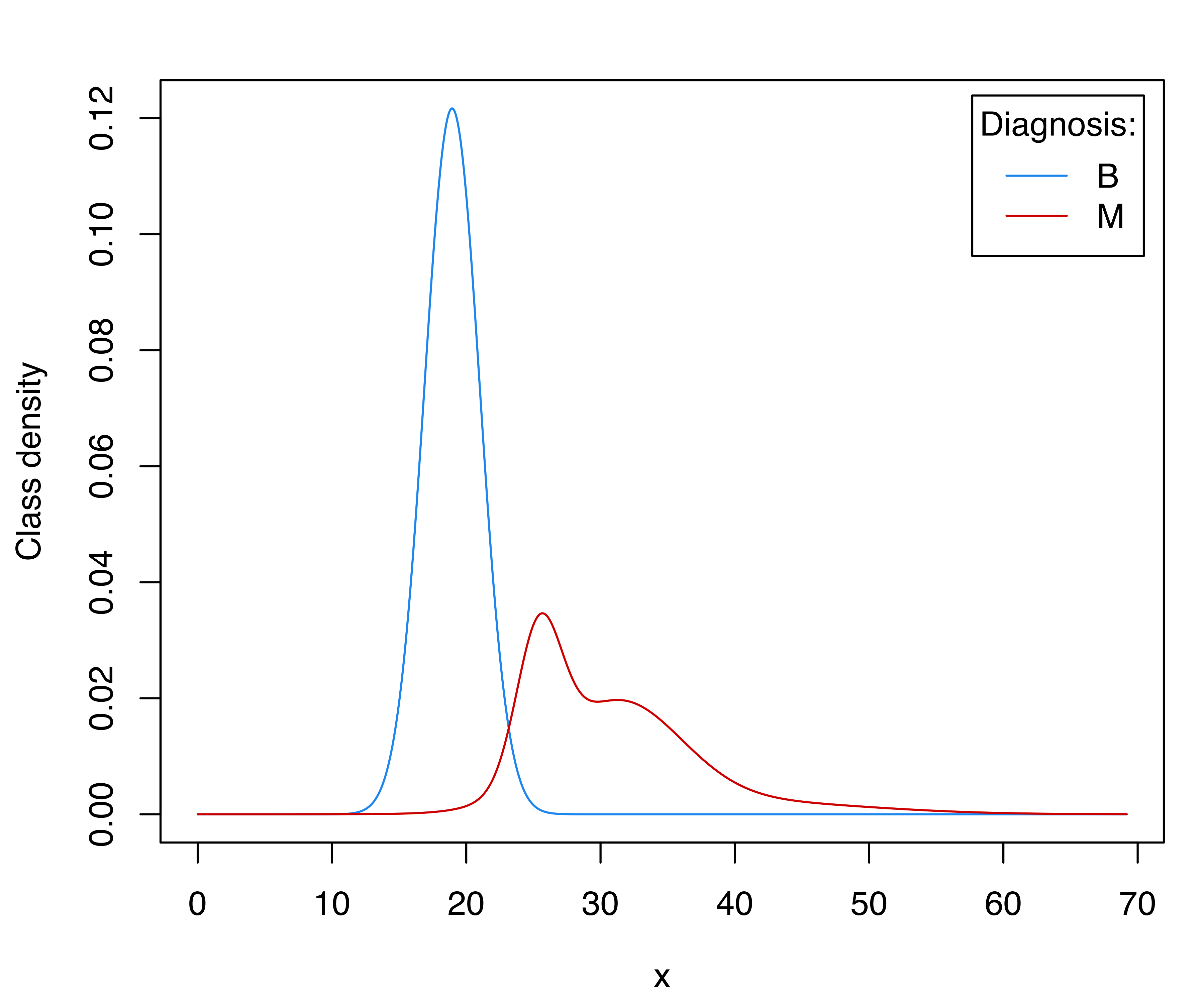
The cross-validated misclassification error for the estimated MclustDA model is obtained as follows:
Adjusting the class prior probabilities, as suggested by Mangasarian, Street, and Wolberg (1995), we get:
Thus, assuming an equal class prior probability, the CV error rate goes down from 3.5% to 2.6%. It is possible to derive the corresponding discriminant thresholds numerically as:
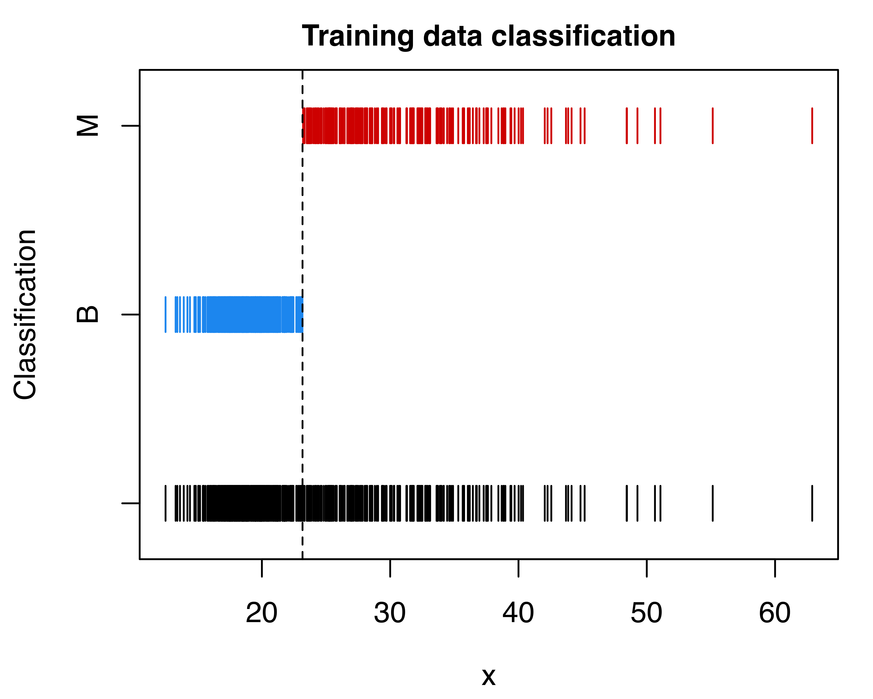
Note that the first threshold is equivalent to the point where the two densities in Figure 4.13 intersect. Using the default discriminant threshold, we can represent the training data graphically with the observed and predicted classes:
plot(mod, what = "scatterplot", main = TRUE)
abline(v = threshold1, lty = 2)
plot(mod, what = "classification", main = TRUE)
abline(v = threshold1, lty = 2)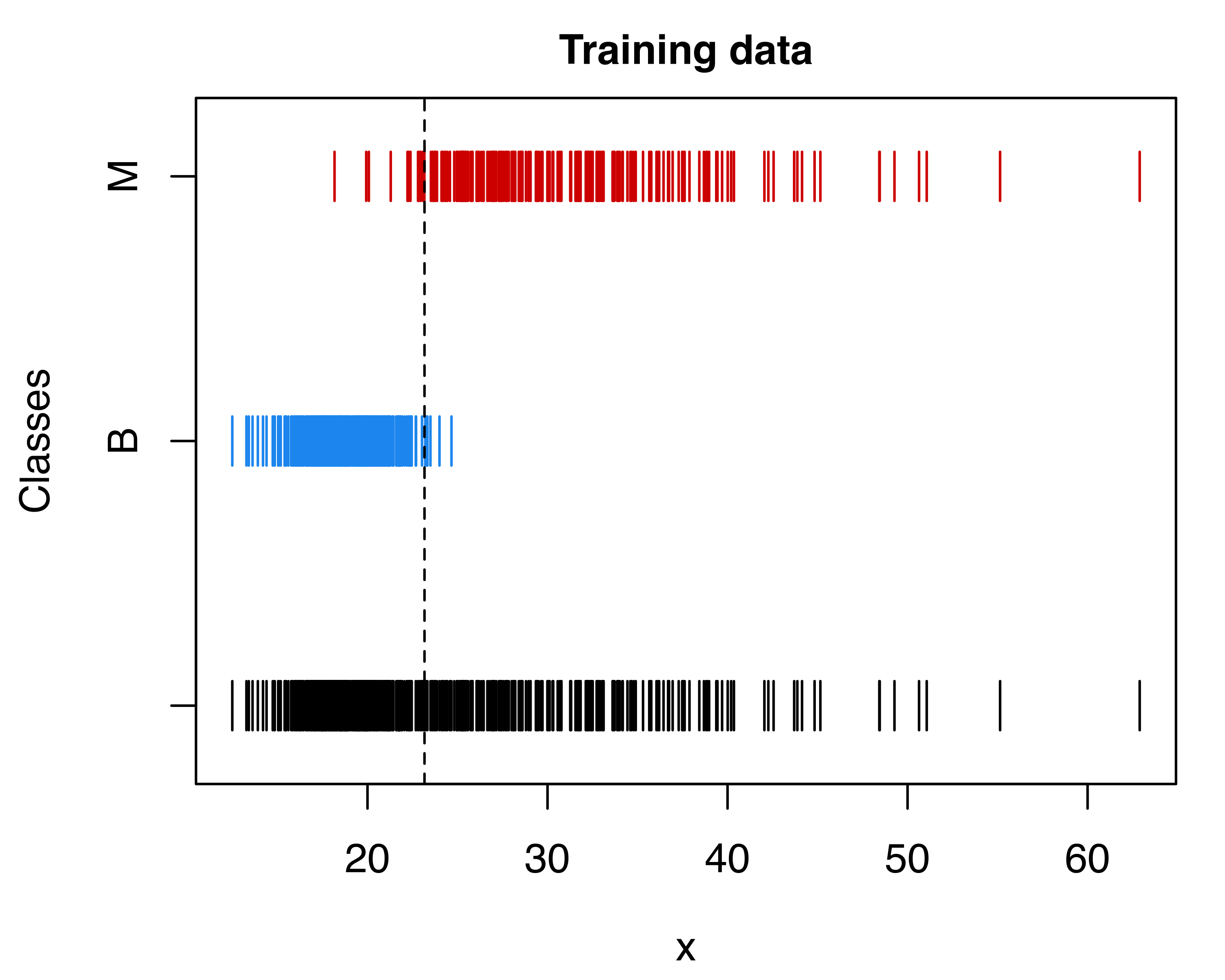
In the search for the optimal classification rule by cross-validation, we can proceed by tuning either the probability threshold for the decision rule or the prior class probabilities. The following code computes and plots the misclassification error rate as a function of the probability threshold used for the classification (see Figure 4.15):
threshold = seq(0.1, 0.9, by = 0.05)
ngrid = length(threshold)
cv = data.frame(threshold, error = numeric(ngrid))
cverr = cvMclustDA(mod, verbose = FALSE)
for (i in seq(threshold))
{
  cv$error[i] = classError(ifelse(cverr$z[, 2] > threshold[i], "M", "B"),
                            Class)$errorRate
}
min(cv$error)
## [1] 0.024605
threshold[which.min(cv$error)]
## [1] 0.35

ggplot(cv, aes(x = threshold, y = error)) +
  geom_point() + geom_line() +
  scale_x_continuous(breaks = seq(0, 1, by = 0.1)) +
  ylab("CV misclassification error") +
  xlab("Probability threshold of malignant (M) tumor class")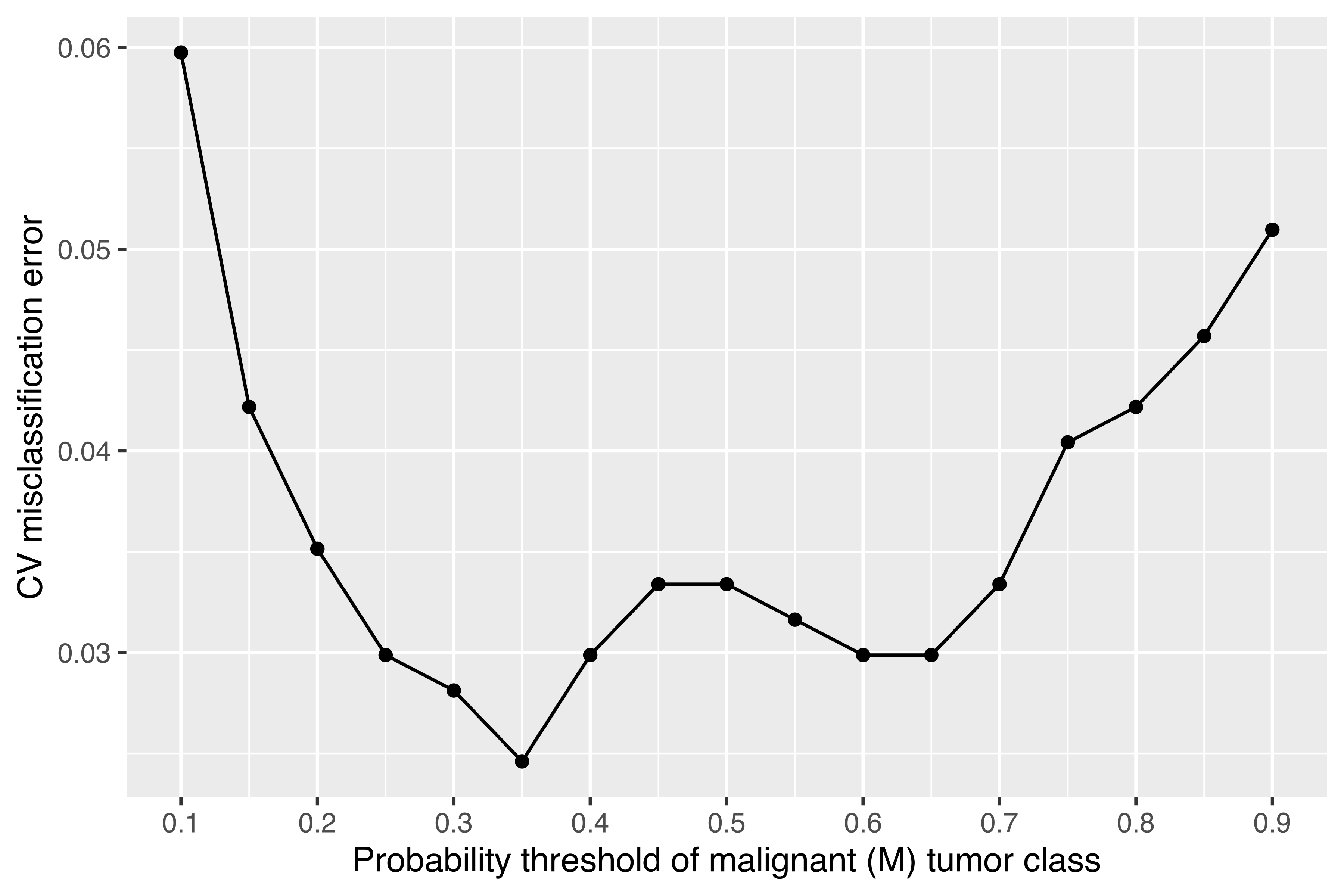
It is thus possible to get a misclassification error of 2.46% by setting the probability threshold to 0.35.
A similar result can also be achieved by adjusting the class prior probabilities. However, because the CV procedure must be replicated for each value specified over a regular grid, this is more computationally demanding. Nevertheless, the added computational effort has the advantage of providing an estimate of the standard error of the CV error estimate itself. This allows us to compute intervals around the CV estimate for assessing the significance of observed differences. The following code computes the CV misclassification error by adjusting the class prior probability of being a malignant tumor, followed by the code for plotting the CV results:
priorProb = seq(0.1, 0.9, by = 0.05)
ngrid = length(priorProb)
cv_error2 = data.frame(priorProb,
                       cv = numeric(ngrid),
                       lower = numeric(ngrid),
                       upper = numeric(ngrid))
for (i in seq(priorProb))
{
  cv = cvMclustDA(mod, prop = c(1-priorProb[i], priorProb[i]),
                  verbose = FALSE)
  cv_error2$cv[i]    = cv$ce
  cv_error2$lower[i] = cv$ce - cv$se.ce
  cv_error2$upper[i] = cv$ce + cv$se.ce
}
min(cv_error2$cv)
## [1] 0.026362
priorProb[which.min(cv_error2$cv)]
## [1] 0.5

ggplot(cv_error2, aes(x = priorProb, y = cv)) +
  geom_point() +
  geom_linerange(aes(ymin = lower, ymax = upper)) +
  scale_x_continuous(breaks = seq(0, 1, by = 0.1)) +
  ylab("CV misclassification error") +
  xlab("Malignant (M) tumor class prior probability")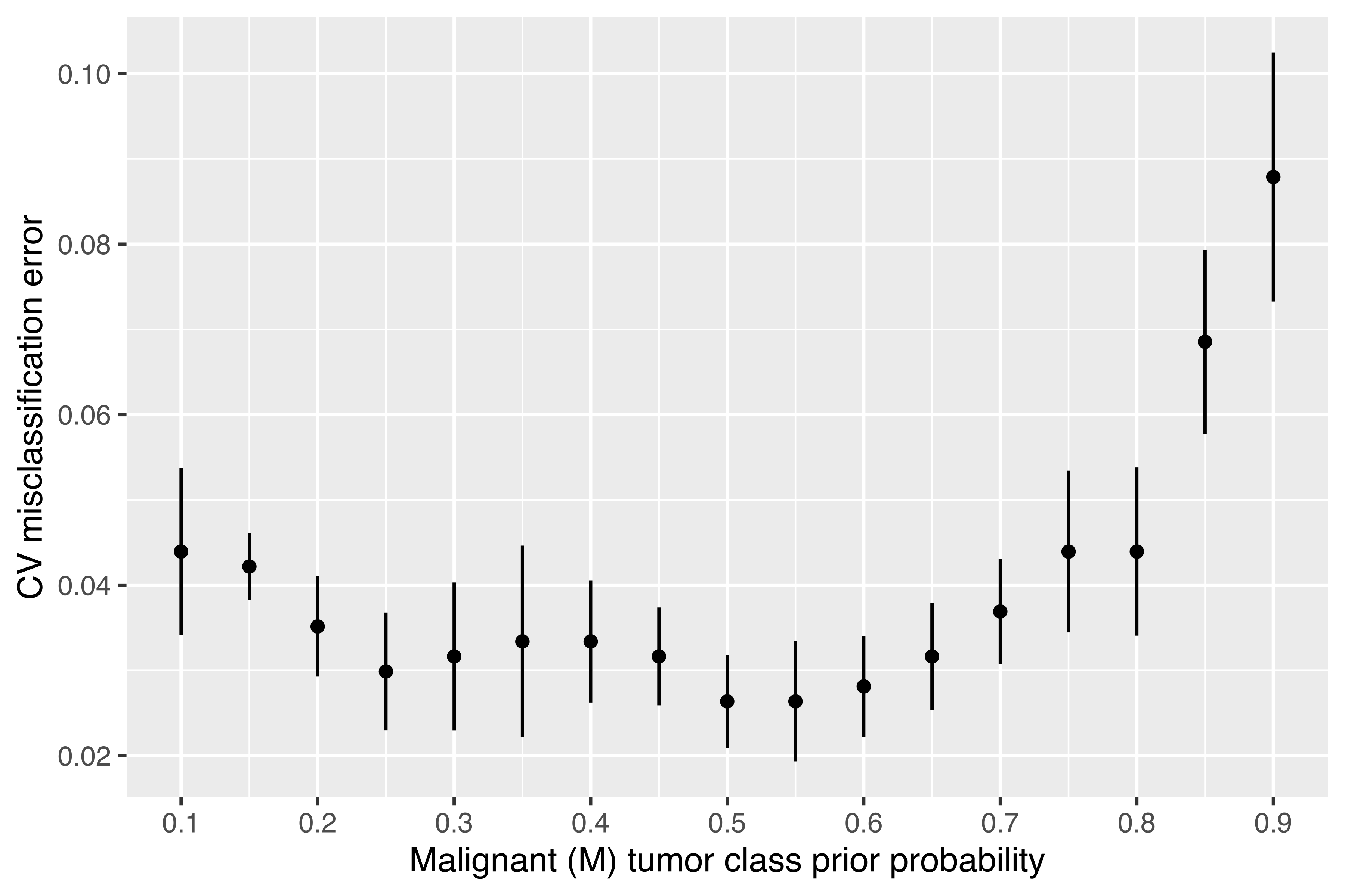
By setting the class prior probabilities at 0.5 each, we get a misclassification error of 2.64%, which is similar to the result obtained by tuning the threshold. The strategy of assuming an equal prior class probability for each breast cancer class adopted by Mangasarian, Street, and Wolberg (1995) appears to be the best approach available.
4.8 Semi-Supervised Classification
Supervised learning methods require knowing the correct class labels for the training data. However, in certain situations the available labeled data may be scarce because they are difficult or expensive to collect, for instance, in anomaly detection, computer-aided diagnosis, drug discovery, and speech recognition. Semi-supervised learning refers to models and algorithms that use both labeled and unlabeled data to perform certain learning tasks [Zhu and Goldberg (2009); VanEngelenHoos:2020]. In classification scenarios, the main goal of semi-supervised learning is to train a classifier using both the labeled and unlabeled data such that its classification performance is better than the one obtained using a classifier trained on the labeled data alone.
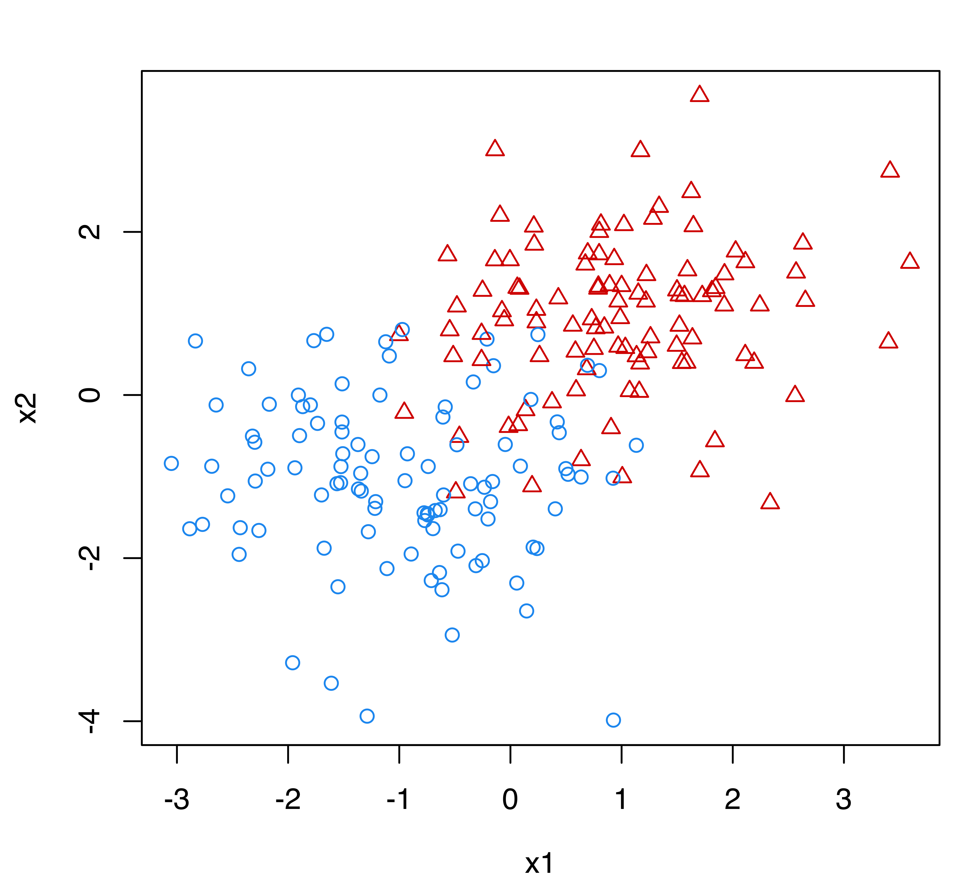
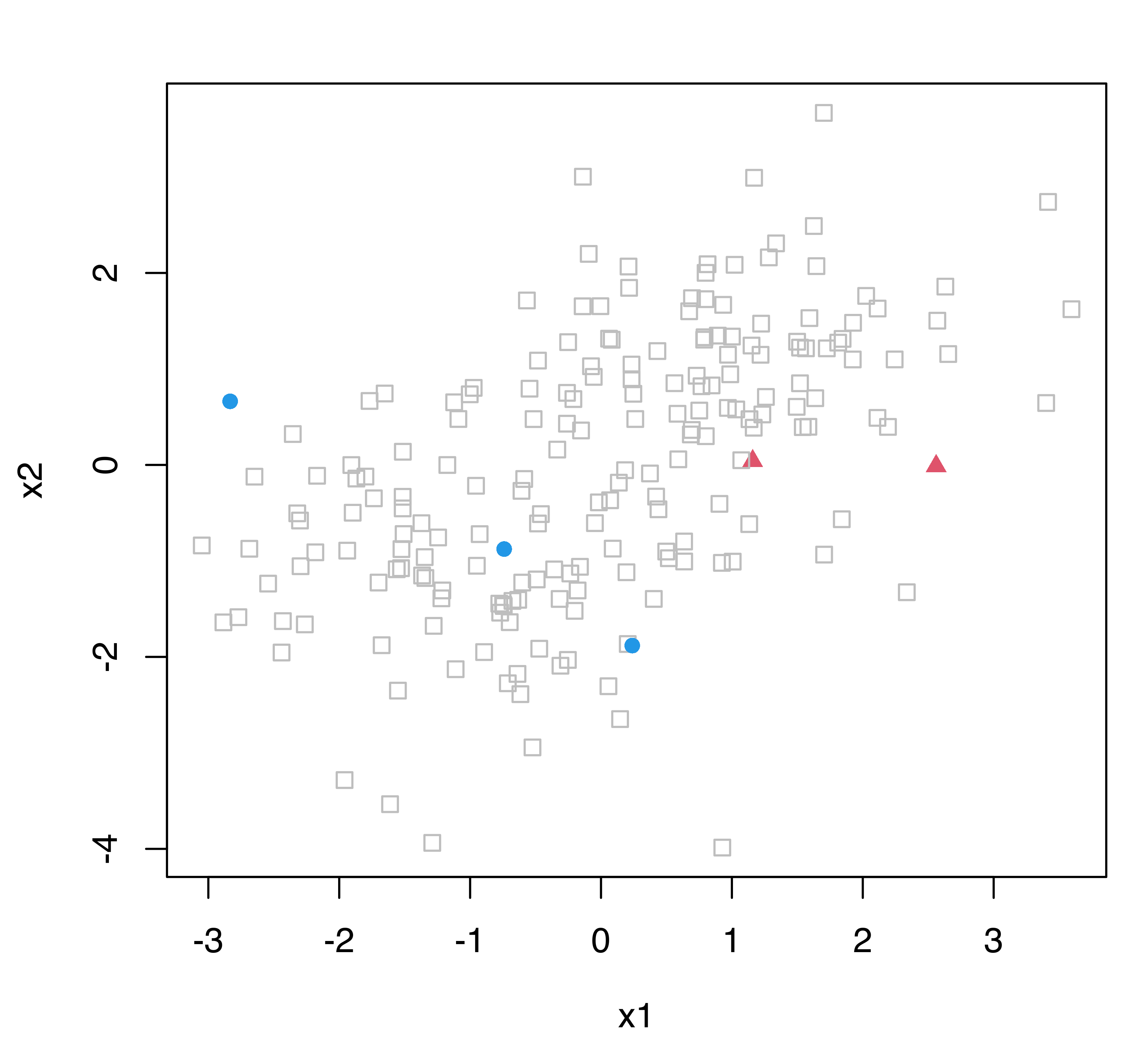
Figure 4.17 shows a simulated two-class dataset with all the observations labeled (see left panel), and with only a few cases labeled (see right panel). In the typical supervised classification setting we would have access to the dataset in Figure 4.17 (a) where labels are available for all the observations. When most of the labels are unknown, as in Figure 4.17 (b), two possible approaches are available. We could use only the (few) labeled cases to estimate a classifier, or we could use both labeled and unlabeled data in a semi-supervised learning approach.
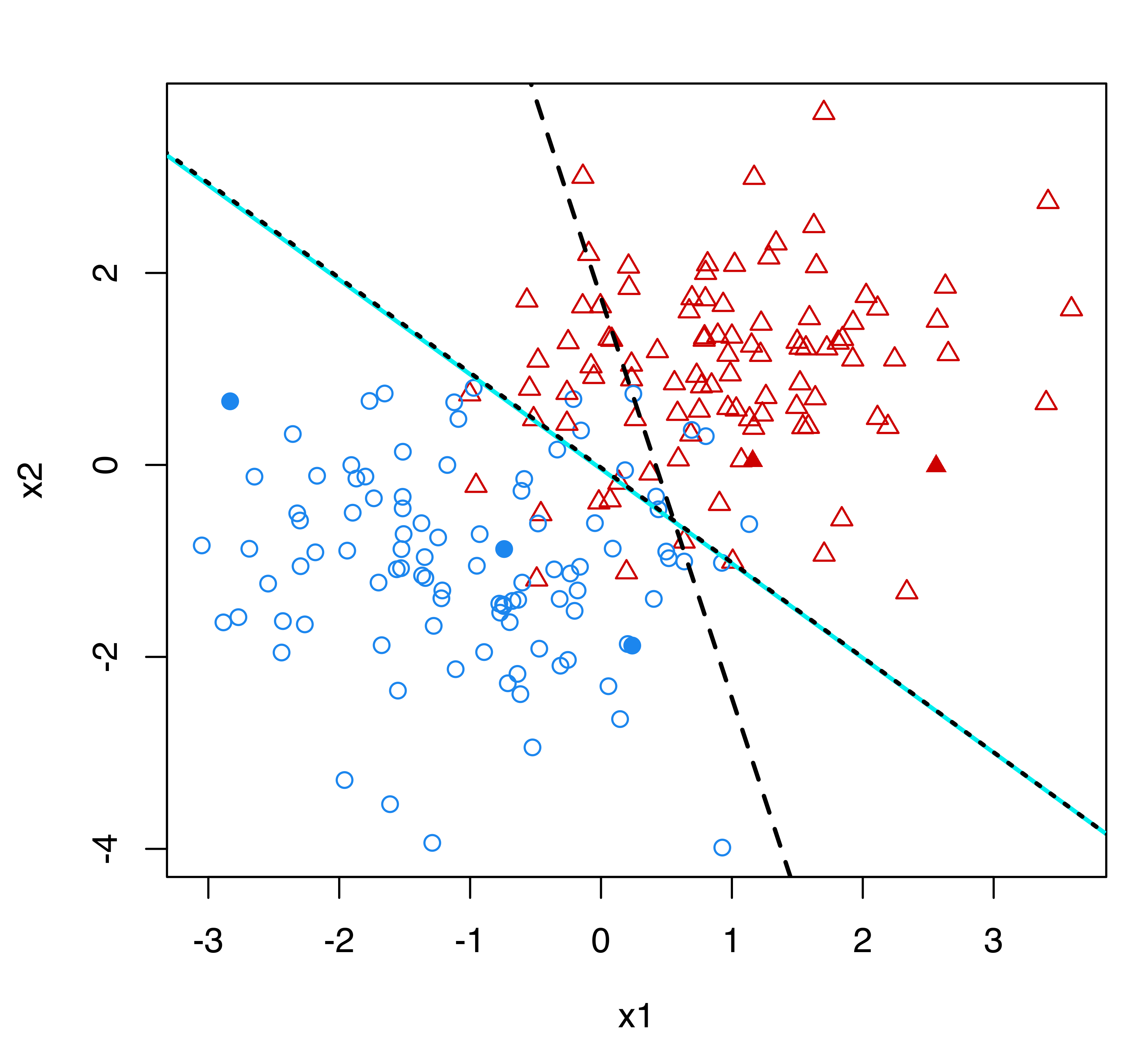
Figure 4.18 shows the classification boundaries corresponding to a supervised classification model estimated under the assumption that the true classes are known (solid line), the boundary for the classification model trained on the labeled data alone (dotted line), and the boundary obtained from a semi-supervised classification model (dashed line). The latter coincides almost exactly with the boundary arising from the full knowledge of class labels. In contrast, the classification boundary from the model estimated using only the labeled data is quite different.
Consider a training dataset \(\mathcal{D}_\text{train}\) made of both \(l\) labeled cases \(\{ (\boldsymbol{x}_i, y_i) \}_{i=1}^l\) and \(u\) unlabeled cases \(\{ \boldsymbol{x}_j \}_{j=l+1}^{n}\), where \(n = l + u\) is the overall sample size. As mentioned earlier, there are usually many more unlabeled than labeled data, so we assume that \(u \gg l\). The likelihood of a semi-supervised mixture model depends on both the labeled and the unlabeled data, so the observed log-likelihood is \[ \ell(\boldsymbol{\Psi}) = \sum_{i=1}^l \sum_{k=1}^K c_{ik} \log\left\{ \pi_k f_k(\boldsymbol{x}_i ; \boldsymbol{\theta}_k) \right\} + \sum_{j=l+1}^{n} \log\left\{ \sum_{g=1}^G \pi_g f_g(\boldsymbol{x}_j ; \boldsymbol{\theta}_g) \right\}, \] where \(c_{ik} = 1\) if observation \(i\) belongs to class \(k\) and \(0\) otherwise. Although in principle the number of components \(G\) can be greater than the number of classes \(K\), it is usually assumed that \(G = K\).
If we treat the unknown labels as missing data, the complete-data log-likelihood can be written as \[\begin{align*} \ell_C(\boldsymbol{\Psi}) = & \sum_{i=1}^l \sum_{k=1}^K c_{ik} \left\{ \log(\pi_k) + \log(f_k(\boldsymbol{x}_i ; \boldsymbol{\theta}_k)) \right\} + \\ & \sum_{j=l+1}^{n} \sum_{g=1}^G z_{jg} \left\{ \log(\pi_g) + \log(f_g(\boldsymbol{x}_j ; \boldsymbol{\theta}_g)) \right\}, \end{align*}\] {#eq-ssmixcloglik} where \(z_{jg} \in (0,1)\) is the conditional probability of observation \(j\) to belong to class \(g\). By assuming a specific parametric distribution for the class and component densities, such as the multivariate Gaussian distribution, the EM algorithm can be used to find maximum likelihood estimates for the unknown parameters of the model. The estimated parameters are then used to classify the unlabeled data, as well as future data. More details can be found in G. J. McLachlan (1977), O’Neill (1978), #McLachlan:Peel:2000 [section 2.19] and Dean, Murphy, and Downey (2006).
mclust provides an implementation for fitting Gaussian semi-supervised classification models through the function MclustSSC(). This requires the input of a data matrix and a vector of class labels, %in which NA with unlabeled data encoded by NA. By default all the available models are fitted and the one with the largest BIC is returned. Optionally, the covariance decompositions described in Section 2.2.1 can be specified via the argument modelNames using the usual nomenclature from Table 2.1. In addition, the optional argument G can be used to specify the number of mixture components. By default, this is set equal to the number of classes from the labeled data.
Example 4.8 Semi-supervised learning of Italian olive oils data
Consider the Italian olive oils dataset available in the pgmm R package (McNicholas et al. 2022). The data are from a study conducted to determine the authenticity of olive oil (Forina et al. 1983) and provide the percentage composition of eight fatty acids found by lipid fraction of 572 Italian olive oils. The olive oils came from nine areas of Italy, which can be further grouped into three regions: Southern Italy, Sardinia, and Northern Italy. The following code reads the data, sets the data frame X of features to build the classifier, and creates the factor class containing the labels for all the observations:
Knowing all the class labels, we can easily fit a discriminant analysis model using the EDDA mixture model discussed in Section 4.2:
mod_EDDA_full = MclustDA(X, class, modelType = "EDDA")
pred_EDDA_full = predict(mod_EDDA_full, newdata = X)
classError(pred_EDDA_full$classification, class)$errorRate
## [1] 0
BrierScore(pred_EDDA_full$z, class)
## [1] 0.00000010836
This model has very good performance, as measured by the classification error and the Brier score, although we must remember that this is an optimistic assessment of model performance because both metrics are computed on the data used for training. Despite this, we can use this performance as a benchmark.
Suppose that only partial knowledge of class labels is available. For instance, we can randomly retain only 10% of the labels as follows:
Since approximately 90% of the data are unlabeled, a semi-supervised classification is called for:
mod_SSC = MclustSSC(X, cl)
plot(mod_SSC, what = "BIC")
mod_SSC$BIC
##      EII    VII    EEI    VEI    EVI    VVI    EEE    VEE    EVE    VVE
## 3 -55641 -55449 -48321 -47813 -47057 -47073 -44348 -44140 -43640 -43323
##      EEV    VEV    EVV    VVV
## 3 -43829 -43539 -43191 -42768
pickBIC(mod_SSC$BIC, 5) - max(mod_SSC$BIC)  # BIC diff for the top-5 models
##   VVV,3   EVV,3   VVE,3   VEV,3   EVE,3
##    0.00 -422.20 -554.53 -770.71 -871.55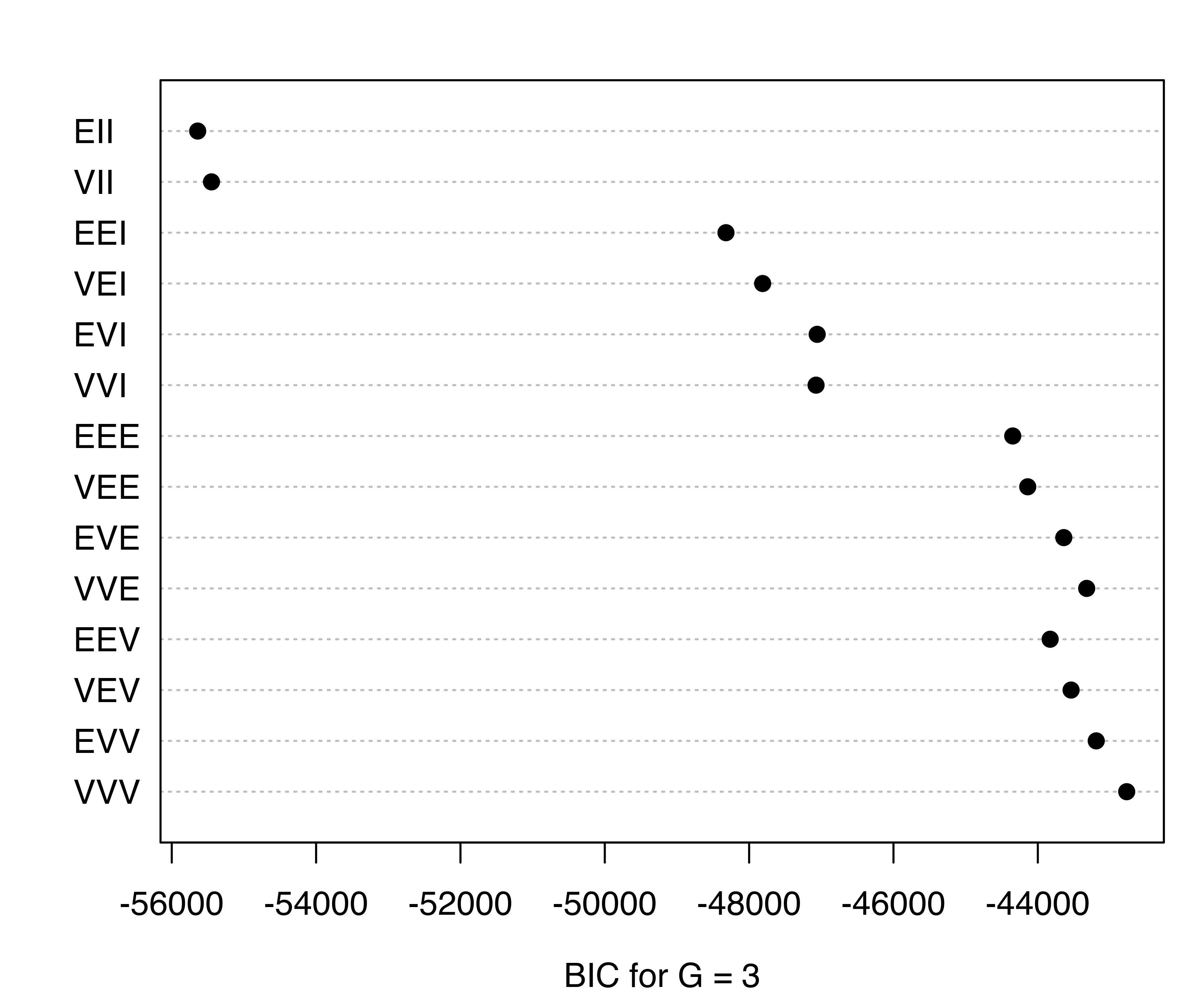
Figure 4.19 plots the BIC values for the models fitted by MclustSSC() with \(G= K = 3\) classes. The best estimated model according to BIC is the unconstrained VVV model. The summary() function can be used to obtain a summary of the fit:
summary(mod_SSC)
## ----------------------------------------------------------------
## Gaussian finite mixture model for semi-supervised classification
## ----------------------------------------------------------------
##
##  log-likelihood   n  df    BIC
##          -20959 572 134 -42768
##
## Classes      n     % Model G
##   South     28  4.90   VVV 1
##   Sardinia  11  1.92   VVV 1
##   North     18  3.15   VVV 1
##   <NA>     515 90.03
##
## Classification summary:
##           Predicted
## Class      South Sardinia North
##   South       28        0     0
##   Sardinia     0       11     0
##   North        0        0    18
##   <NA>       295       86   134
We can evaluate the estimated classifier by comparing the predicted classes with the true classes for the unlabeled observations:
pred_SSC = predict(mod_SSC, newdata = X[is.na(cl), ])
table(Predicted = pred_SSC$classification, Class = class[is.na(cl)])
##           Class
## Predicted  South Sardinia North
##   South      295        0     0
##   Sardinia     0       86     0
##   North        0        1   133
classError(pred_SSC$classification, class[is.na(cl)])$errorRate
## [1] 0.0019417
BrierScore(pred_SSC$z, class[is.na(cl)])
## [1] 0.0019417
The performance appears quite good with only one unlabeled observation misclassified.
We now compare the semi-supervised approach with the classification approach that uses only the labeled data, as a function of the percentage of full data information. The following code implements this comparison using the Brier score as performance metric:
pct_labeled_data = c(5, seq(10, 90, by = 10), 95)
BS = matrix(as.double(NA), nrow = length(pct_labeled_data), ncol = 2,
             dimnames = list(pct_labeled_data, c("EDDA", "SSC")))
for (i in seq(pct_labeled_data))
{
  cl = class
  labeled = sample(1:n, round(n*pct_labeled_data[i]/100))
  cl[-labeled] = NA
  # Classification on labeled data
  mod_EDDA  = MclustDA(X[labeled, ], cl[labeled],
                        modelType = "EDDA")
  # prediction for the unlabeled data
  pred_EDDA = predict(mod_EDDA, newdata = X[-labeled, ])
  BS[i, 1]  = BrierScore(pred_EDDA$z, class[-labeled])
  # Semi-supervised classification
  mod_SSC  = MclustSSC(X, cl)
  # prediction for the unlabeled data
  pred_SSC = predict(mod_SSC, newdata = X[-labeled, ])
  BS[i, 2] = BrierScore(pred_SSC$z, class[-labeled])
}
BS
##                   EDDA                 SSC
## 5  0.36757342343703858 0.00184075724060626
## 10 0.14649511848830127 0.00194083725139750
## 20 0.00000004794698661 0.00218238248453443
## 30 0.00500200204812944 0.00000000044264099
## 40 0.00356335895644648 0.00000009331253357
## 50 0.01740046202639491 0.00349653566200317
## 60 0.00000033388757151 0.00000014123579678
## 70 0.00585344025094451 0.00000037530321144
## 80 0.00002069320555273 0.00000027964277368
## 90 0.00000000012729332 0.00000000000499843
## 95 0.00000000000069483 0.00000000000052263

matplot(pct_labeled_data, BS, type = "b",
        lty = 1, pch = c(19, 15), col = c(2, 4), xaxt = "n",
        xlab = "Percentage of labeled data", ylab = "Brier score")
axis(side = 1, at = pct_labeled_data)
abline(h = BrierScore(pred_EDDA_full$z, class), lty = 2)
legend("topright", pch = c(19, 15), col = c(2, 4), lty = 1,
       legend = c("EDDA", "SSC"), inset = 0.02)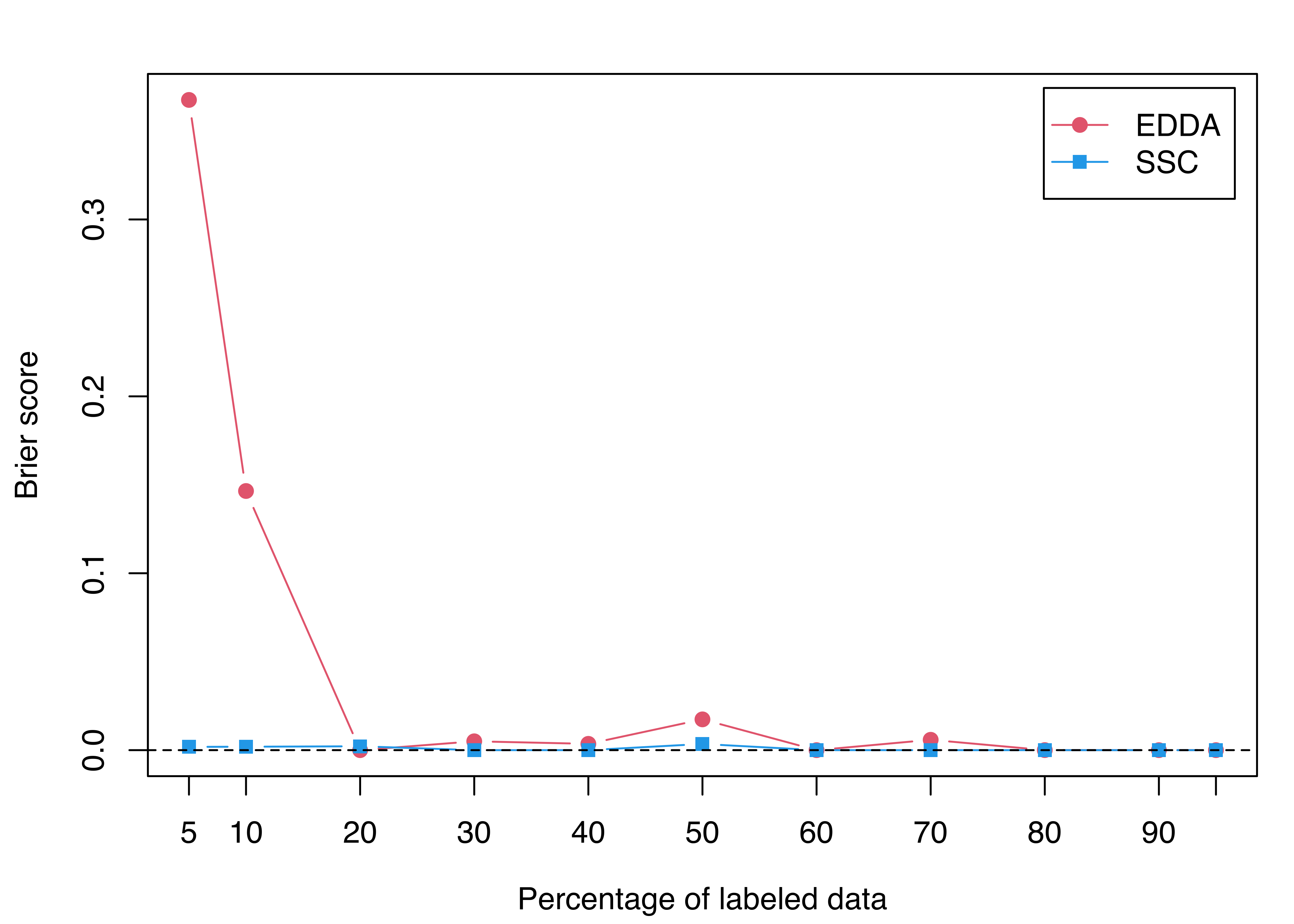
Looking at the table of results and Figure 4.20, it is clear that EDDA requires a large percentage of labeled data to achieve a reasonable performance. In contrast, the semi-supervised classification (SSC) model is able to achieve almost perfect classification accuracy with a very small portion of labeled data.
In stratified cross-validation the data are randomly split in such a way that maintains the same class distribution in each fold. This is of particular relevance in the case of unbalanced class distribution. Furthermore, it has been noted that “stratification is generally a better scheme, both in terms of bias and variance, when compared to regular cross-validation” (Kohavi 1995).↩︎